Working with waveforms
This page provides an introduction to the contents of waveforms dataframes. Please refer to Working with flights for details on how to load waveform data for a flight.
The documentation below assumes you’ve already loaded waveform data into a variable called “frame”.
The waveform dataframe contains a large number of columns. Initially, the frame will contain 24 columns:
>>> frame.columns
Index(['bias_rx', 'bias_tx', 'channel', 'digitizer', 'ins_alt', 'ins_east',
       'ins_heading', 'ins_lat', 'ins_lon', 'ins_north', 'ins_pitch',
       'ins_roll', 'ins_zone', 'pulse_count', 'pulse_number', 'range',
       'raster_number', 'rx', 'scan_angle', 'thresh_rx', 'thresh_tx', 'time',
       'tx', 'waveform_count'],
       dtype='object')
These fields come from two different sources: the TLD files which contain the waveform data and the INS trajectory which contains position and attitude data. The INS fields are all prefixed with “ins” for clarity.
The return waveforms are in the rx field. (The tx field contains transmit waveforms.) If you have matplotlib, you can plot the return waveform for an individual record (in this case, 116) like so:
>>> import matplotlib.pyplot as plt
>>> plt.plot(frame.rx[116])
[<matplotlib.lines.Line2D object at 0x7f02c00e4278>]
>>> plt.show()
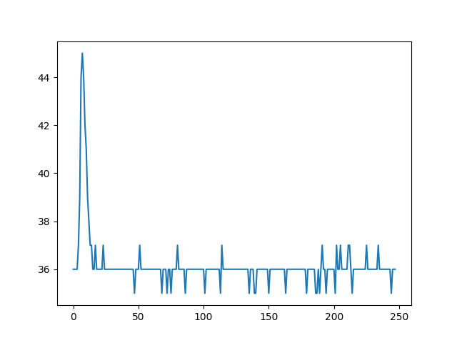
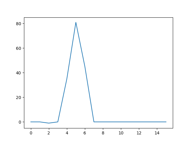
The range of the sample values is 0 to 255. However, the digitizers pick up a level of background energy so the baseline of the waveform will always be higher than 0. In this case, it’s at about 36. You might find it helpful to remove the background energy by removing the value of the first sample, like so:
>>> plt.plot(frame.rx[116] - frame.rx[116][0])
[<matplotlib.lines.Line2D object at 0x7f02c004d4e0>]
>>> plt.show()

If you like, you can also similarly visualize the transmit waveform:
>>> plt.plot(frame.tx[116] - frame.tx[116][0])
[<matplotlib.lines.Line2D object at 0x7f02bbde64a8>]
>>> plt.show()
The library contains some basic methods for waveform analysis and derivation of a point cloud. The basic workflow for EAARL-B looks like this:
>>> import eaarl.analyze
>>> frame = eaarl.analyze.remove_failed_thresh(frame)
>>> frame = eaarl.analyze.add_mirror(frame, flight.ops)
>>> frame = eaarl.analyze.add_fs(frame, flight.ops)
>>> frame.columns
Index(['bias_rx', 'bias_tx', 'channel', 'digitizer', 'ins_alt', 'ins_east',
       'ins_heading', 'ins_lat', 'ins_lon', 'ins_north', 'ins_pitch',
       'ins_roll', 'ins_zone', 'pulse_count', 'pulse_number', 'range',
       'raster_number', 'rx', 'scan_angle', 'thresh_rx', 'thresh_tx', 'time',
       'tx', 'waveform_count', 'tx_pos', 'mir_x', 'mir_y', 'mir_z', 'fs_pos',
       'fs_range', 'fs_x', 'fs_y', 'fs_z'],
       dtype='object')
We start by using remove_failed_thersh to remove records where the hardware sensor indicates that the transmit or waveform failed a hardware-defined threshold (the thresh_tx and thresh_rx fields). This step is optional, but was always used for production data in ALPS.
Then add_mirror adds the fields tx_pos, mir_x, mir_y, and mir_z. These represent the position in the transmit waveform of the centroid and the x,y,z location of the oscillating scan mirror in UTM cooordinates.
Finally, add_fs add the fields fs_pos, fs_range, fs_x, fs_y, and fs_z. These represent the position in the return waveform of the surface centroid, the range in meters between the scan mirror and the detected target, and the x,y,z, location of the target in UTM coordinates.
If you are working with EAARL-A data, then an additional step is required. In the EAARL-A system, all three channels represent the same point. They each receive a different amount of the return energy, allowing for a greater range of sensitivity. You need to select the first non-saturated return for each pulse using select_eaarla_channel. The revised workflow looks like this:
>>> import eaarl.analyze
>>> frame = eaarl.analyze.remove_failed_thresh(frame)
>>> frame = eaarl.analyze.select_eaarla_channel(frame)
>>> frame = eaarl.analyze.add_mirror(frame, flight.ops)
>>> frame = eaarl.analyze.add_fs(frame, flight.ops)
If you prefer to keep all three EAARL-A channels available or would like to create your own algorithm for selecting which channel to use, then you should manually remove channel 4 which contains noise:
>>> frame = frame[frame.channel != 4]
Here’s an example that plots the detected surfaces in matplotlib for a frame that contains a single raster:
>>> from mpl_toolkits.mplot3d import Axes3D
>>> fig = plt.figure()
>>> ax = fig.add_subplot(111, projection='3d')
>>> ax.scatter(frame.fs_x, frame.fs_y, frame.fs_z)
<mpl_toolkits.mplot3d.art3d.Path3DCollection object at 0x7f02c02ea748>
>>> plt.show()

The point data will often contain outliers. The library implements the gridded RCF which can help detect them. The function rcf_grid will return an array of booleans where True indicates the record passed and False indicates it failed. Here is an example that detects points that pass the filter using a 15m vertical search window and a 5m horizontal cell size:
>>> import eaarl.rcf
>>> good = eaarl.rcf.rcf_grid(frame.fs_x, frame.fs_y, frame.fs_z, 15, 5)
>>> len(frame)
424
>>> len(frame[good])
382