Important
This ShakeMap 3.5 Manual is deprecated. Please see the ShakeMap 4 Manual.
2.5. ShakeMap Processing
As discussed in the User’s Guide, ShakeMap produces a range of output products. However, ShakeMap’s primary outputs are grids of interpolated ground motions, from which the other grids, contours, and maps are derived. Interpolated grids are produced for PGA, PGV, macroseismic intensity (we will hereafter refer to macroseismic intensity as “MMI” for Modified Mercalli Intensity, but other intensity measures are supported), and (optionally) pseudo-spectral accelerations at 0.3, 1.0, and 3.0 sec. Attendant grids of shaking-parameter uncertainty and Vs30, are also produced as separate products or for later analyses of each intermediate processing step, if so desired.
The ShakeMap program responsible for producing the interpolated grids is called “grind”. This section is a description of the way grind works, and some of the configuration parameters and command-line flags that control specific functionality. (For a complete description of configuring and running grind, see the Software Guide and the configuration file grind.conf.)
Below is an outline of the ShakeMap processing workflow. Figure 1 provides a schematic of the key processing steps.
Data Preparation
Remove flagged stations
Convert intensities to peak ground motions (PGMs) and vice versa
Correct data to “rock” using Vs30-based amplification terms
Remove estimated basin response (optional)
Correct earthquake bias with respect to the chosen GMPE
Remove the effect of directivity (optional)
Compute bias
Flag outliers
Repeat the previous two steps until no outliers are found
Create bias-adjusted GMPE estimates at each station location and for the entire output grid (optionally, apply directivity)
Interpolate ground motions to a uniform grid
Amplify ground motions
Basin amplifications (optional)
Vs30 site amplifications
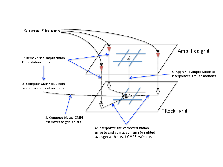
Figure 1: A schematic of the basic ShakeMap ground motion interpolation scheme.
The sections that follow provide a more complete description of the processing steps outlined above.
2.5.1. Data preparation
The first step in processing is the preparation of the parametric data. As discussed in the Software Guide, ground motion amplitudes are provided to ShakeMap in the form of Extended Markup Language (XML) files. Note that we describe here the behavior of grind with respect to the input XML file(s). The programs that produce the input XML (be it db2xml, others, or the network operator’s custom codes) will have their own rules as to what is included in the input.
In our presentation here, the term “station” refers to a single seismographic station denoted with a station ID (i.e., a code or number). In current practice, station IDs often consist of a network identifier concatenated (using a “.”) with the station ID (e.g., “CI.JVC” or “CE.50281”).
Each station may have one or more “channels,” each of which is denoted by an ID code (often called a “seedchan”). The last character of the ID is assumed to be the orientation of the instrument (east-west, north-south, vertical). ShakeMap only uses the peak horizontal component. Thus, ShakeMap does not consider amplitudes with a “Z” as the final character, though it does carry the vertical amplitude values through to the output station files. Note that some stations in some networks are given orientations of “1”, “2”, and “3” (rather than the more standard “N”, “E”, and “Z”), where any of the components may be vertical. Because of the non-standardized nature of these component labels, ShakeMap does not attempt to discern their orientation and assumes that they are all horizontal. This can lead to inaccuracies—it becomes the network operator’s responsibility to ensure that the vertical channel is either excluded or labeled with a “Z” before the data are presented to ShakeMap. Similarly, many networks co-locate broadband instruments with strong-motion instruments and produce PGMs for both. Again, it is the network operator’s responsibility to select the instrument that best represents the data for the PGMs in question. Aside from the station flagging discussed below, ShakeMap makes no attempt to discern which of a set of components is superior, it will simply use the largest value it finds (i.e., if ShakeMap sees channels “HNE” and “HHE” for the same station, it will simply use the larger of the two PGMS without regard to the possibility that one may be off-scale or below-noise).
Currently, ShakeMap is location-code agnostic. Because the current SNCL (Station, Network, Channel, Location) specification defines the location code as a pure identifier (i.e., it should have no meaning), it is impossible to anticipate all the ways it may be used. Therefore, if a network-station combo has multiple instruments at multiple locations, the data provider should identify each location as a distinct station for ShakeMap XML input purposes (by, for example, including the location code as part of the station identifier, N.S.L—e.g., ‘CI.JVC.01’). If the network uses the location codes in another manner, it is up to the operator to generate a station/component data structure that ShakeMap will handle correctly.
Finally, each channel may produce one or more amplitudes (e.g., PGA, PGV, pseudo- spectral acceleration). Note that these amplitudes should always be supplied by the network as positive values, regardless of the direction of the peak motion. The amplitudes for all stations and channels are collected and reported, but only the peak horizontal amplitude of each ground-motion parameter is used by ShakeMap.
The foregoing is not intended to be a complete description of the requirements for the input data. Please see the relevant section of the Software Guide for complete information.
2.5.1.1. Flagged Stations
If the “flag” attribute of any amplitude in the input XML is non-null and non-zero, then all components of that station are flagged as unusable. The reasoning here is that for a given data stream, the typical network errors (telemetry glitch, incomplete data, off-scale or below-noise data, etc.) will affect all of the parameters (as they are typically all derived from the same data stream), and it is therefore impossible to determine the peak horizontal component of any ground-motion parameter. This restriction is not without its detractors, however, and we may revisit it at a future date.
MMI data are treated in much the same way; however, there is typically only one “channel” and one parameter (i.e., intensity).
ShakeMap presents flagged stations as open, unfilled triangles on maps and on regression plots. In contrast, unflagged stations are color coded by network or, optionally, by their amplitudes via their converted intensity value, as shown in Figure 2. Flagged stations are also indicated as such within tables produced for ShakeMap webpage consumption, e.g., the stations.xml file.

Figure 2: Peak acceleration ShakeMap from the Aug. 24, 2014, M6.0 American Canyon (Napa Valley), California earthquake. Strong motion data (triangles) and intensity data (circles) are color-coded according to their intensity value, either as observed (for macroseismic data) or as converted by Wald et al. (1999b) as shown in the legend. The north-south black line indicates the fault location, which nucleated near the epicenter (red star). Note: Map Version Number reflects separate offline processing for this Manual.
2.5.1.2. Converting MMI to PGM and PGM to MMI
Once the input data have been read and peak amplitudes assigned for each station (which may be null if the data are flagged), intensities are derived from the peak amplitudes and peak amplitudes are derived from the intensities using the GMICEs configured (see the parameters ‘pgm2mi’ and ‘mi2pgm’ in grind.conf). Small values of observed intensities (MMI < III for PGA, and MMI < IV for other parameters) are not converted to PGM for inclusion in the PGM maps. Our testing indicated that including these low intensities introduced a significant source of error in the interpolation, likely due to the very wide range (and overlap) of ground motions that can produce MMIs lower than III or IV.
2.5.1.3. Site Corrections
Near-surface conditions can have a substantial effect on ground motions. Ground motions at soft-soil sites, for instance, will typically be amplified relative to sites on bedrock. Because we wish to interpolate sparse data to a grid over which site characteristics may vary greatly, we first remove the effects of near-surface amplification from our data, perform the interpolation to a uniform grid at bedrock conditions, and then apply the site amplifications to each point in the grid, based on each site’s characteristics.
A commonly used proxy used to account for site effects (e.g., Borcherdt, 1994) is Vs30, the time-averaged shear wave velocity to 30 meters depth. Vs30 is also a fundamental explanatory variable for modern GMPEs (e.g., Abrahamson et al., 2014). Since the use of GMPEs for ground motion estimation is fundamental to ShakeMap, we follow this convention and use Vs30-based amplification terms to account for site amplification. In Future Directions, we suggest alternative approaches that require additional site information beyond Vs30.
2.5.1.3.1. Site Characterization Map
Each region wishing to implement ShakeMap should have a Vs30 map that covers the entire area they wish to map. Using the Jan. 17, 1994, M6.7 Northridge, California earthquake ShakeMap as an example (Figure 3), we present, in Figure 4, the Vs30 map used. Until 2015, the California site-condition map was based on geologic base maps as introduced by Wills et al. (2000), and modified by Howard Bundock and Linda Seekins of the USGS at Menlo Park (H. Bundock, written comm., 2002). The Wills et al. map extent is that of the State boundary; however, ShakeMap requires a rectangular grid, so fixed velocity regions were inserted to fill the grid areas representing the ocean and land outside of California. Unique values were chosen to make it easy to replace those values in the future. The southern boundary of the Wills et al. map coincides with the U.S.A./Mexico border. However, due to the abundant seismic activity in Imperial Valley and northern Mexico, we have continued the trend of the Imperial Valley and Peninsular Ranges south of the border by approximating the geology based on the topography; classification BC was assigned to sites above 100m in elevation and CD was assigned to those below 100m. This results in continuity of our site correction across the international border.
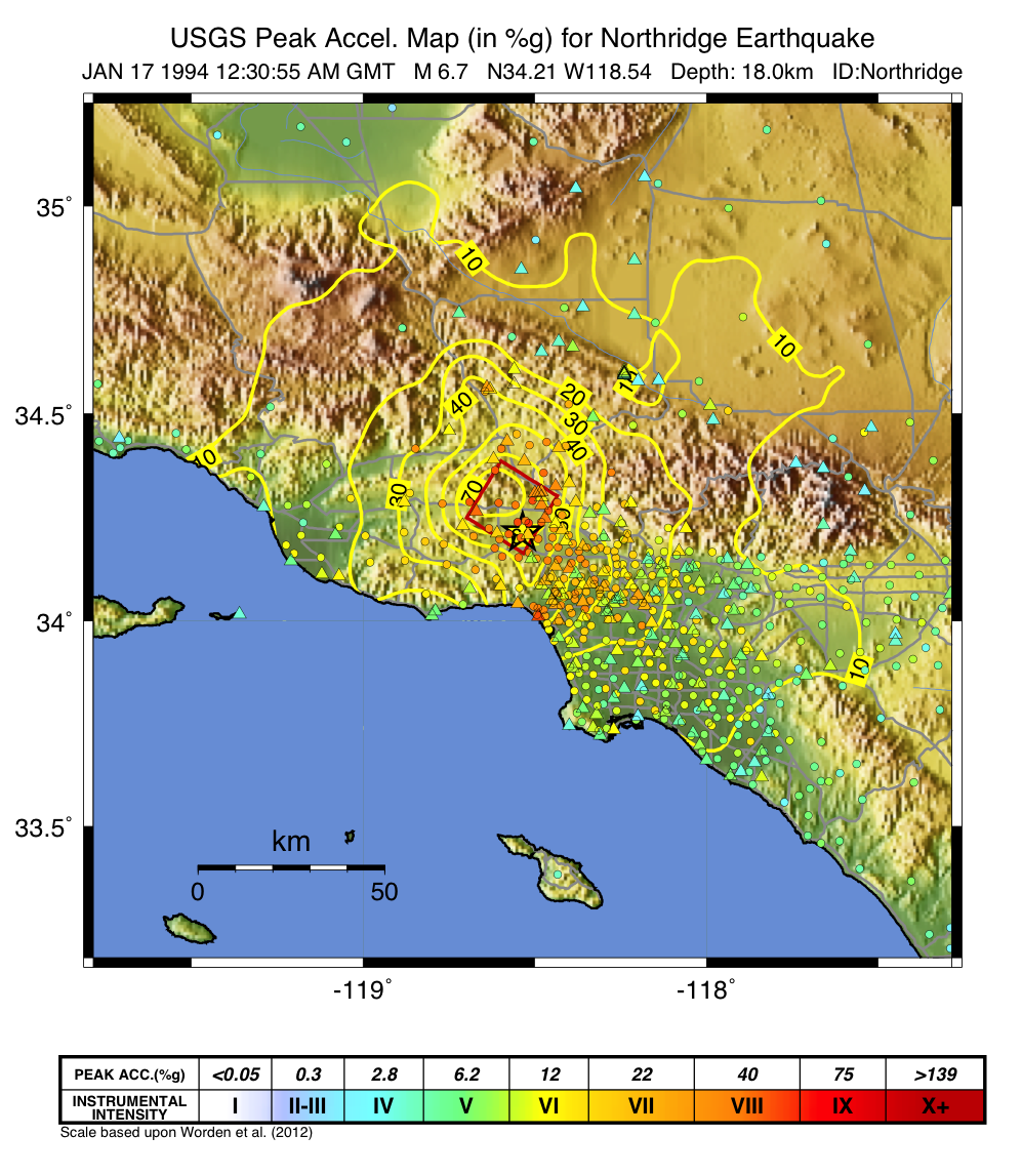
Figure 3: PGA ShakeMap reprocessed with data from the 1994 M6.7 Northridge, CA earthquake with a finite fault (red rectangle), strong motion data (triangles), and intensity data (circles). Stations and macroseismic data are color-coded according to their intensity value, either as observed (for macroseismic data) or as converted by Worden et al. (2012) and indicated by the scale shown.
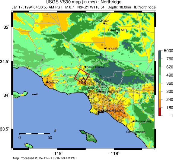
Figure 4: Vs30 Map produced as a byproduct of ShakeMap for the 1994 M6.7 Northridge, CA earthquake. The finite fault is shown as a red rectangle; strong motion data (triangles) and intensity data (circles) are transparent to see site conditions. The legend indicates the range of color-coded Vs30 values in m/sec.
Other ShakeMap operators have employed existing geotechnically- or geologically-based Vs30 maps, or have developed their own Vs30 map for the area covered by their ShakeMap. For regions lacking such maps, including most of globe, operators often employ the approach of Wald and Allen (2007), revised by Allen and Wald, (2009b), which provides estimates of Vs30 as a function of more readily available topographic slope data. Wald and Allen’s slope-based Vs30-mapping proxy is employed by the Global ShakeMap (GSM) system.
Recent developments by Wald et al. (2011d) and Thompson et al. (2012; 2014) provide a basis for refining Vs30 maps when Vs30 data constraints are abundant. Their method employs not only geologic units and topographic slope, but also explicitly constrains map values near Vs30 observations using kriging-with-a-trend to introduce the level of spatial variations seen in the Vs30 data (Thompson et al., 2014). An example of Vs30 for California using this approach is provided in Figure 5. Thompson et al. describe how differences among Vs30 base maps translate into variations in site amplification in ShakeMap.
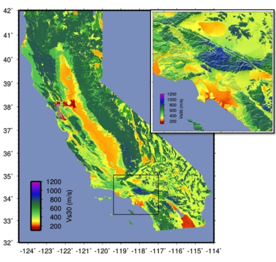
Figure 5: Revised California Vs30 Map (Thompson et al., 2014). This map combines geology, topographic slope, and constraints of map values near Vs30 observations using kriging-with-a-trend. Inset shows Los Angeles region, with Los Angeles Basin indicating low Vs30 velocities.
Worden et al. (2015) further consolidate readily available Vs30 map grids used for ShakeMaps at regional seismic networks of the ANSS with background, Thompson et al.’s California Vs30 map, and the topographic-based Vs30 proxy to develop a consistently scaled mosaic of Vs30 maps for the globe with smooth transitions from tile to tile. It is anticipated that aggregated Vs30 data provided by Yong et al. (2015) will facilitate further map development of other portions of the U.S.
2.5.1.3.2. Amplification Factors
ShakeMap provides two operator-selectable methods for determining the factors used to amplify and de-amplify ground motions based on Vs30. The first is to apply the frequency- and amplitude-dependent factors, such as those determined by Borcherdt (1994) or Seyhan and Stewart (2014). By default, amplification of PGA employs Borcherdt’s short-period factors; PGV uses mid-period factors; and PSA at 0.3, 1.0, and 3.0 sec uses the short-, mid-, and long-period factors, respectively. The second method uses the site correction terms supplied with the user’s chosen GMPE (if such terms are supplied for that GMPE). The differences between these choices and their behavior with respect to other user-configurable parameters are discussed in the Software & Implementation Guide.
2.5.1.3.3. Correct Data to “Rock”
If, as is usually the case, the operator has opted to apply site amplification (via the -qtm option to grind), the ground-motion observations are corrected (de-amplified) to “rock”. (The Vs30 of “rock” is specified with the parameter ‘smVs30default’ in grind.conf.) See the section “Site Corrections” in the Software Guide for a complete discussion of the way site amplifications are handled and the options for doing so.
Note that Borcherdt-style corrections do not handle PGV directly, so PGV is converted to 1.0 sec PSA (using Newmark and Hall, 1982), (de)amplified using the mid-period Borcherdt terms, and then converted back to PGV. The Newmark and Hall conversion is entirely linear and reversible, so while the conversion itself is an approximation, no bias or uncertainty remains from the conversion following a “round trip” from site to bedrock back to site.
Because there are no well-established site correction terms for MMI, when Borcherdt- style corrections are specified, ShakeMap converts MMI to PGM, applies the (de)amplification to PGM using the Borcherdt terms, then converts the PGMs back to MMI.
Figure 6 and Figure 7 show shaking estimates (for PGA and MMI, respectively) before site correction (upper left) and after (upper right). Without site correction, ground motion attenuation is uniform as a function of hypocentral distance (in the absence of a finite fault model as in panels A through C) and fault distance (as in D); with site correction, the correlation of amplitudes with the Vs30 map (and also topography) are more apparent. This distinction is important: often complexity in ShakeMap’s peak ground motions and intensity patterns are driven by site terms, rather than variability due to shaking observations.
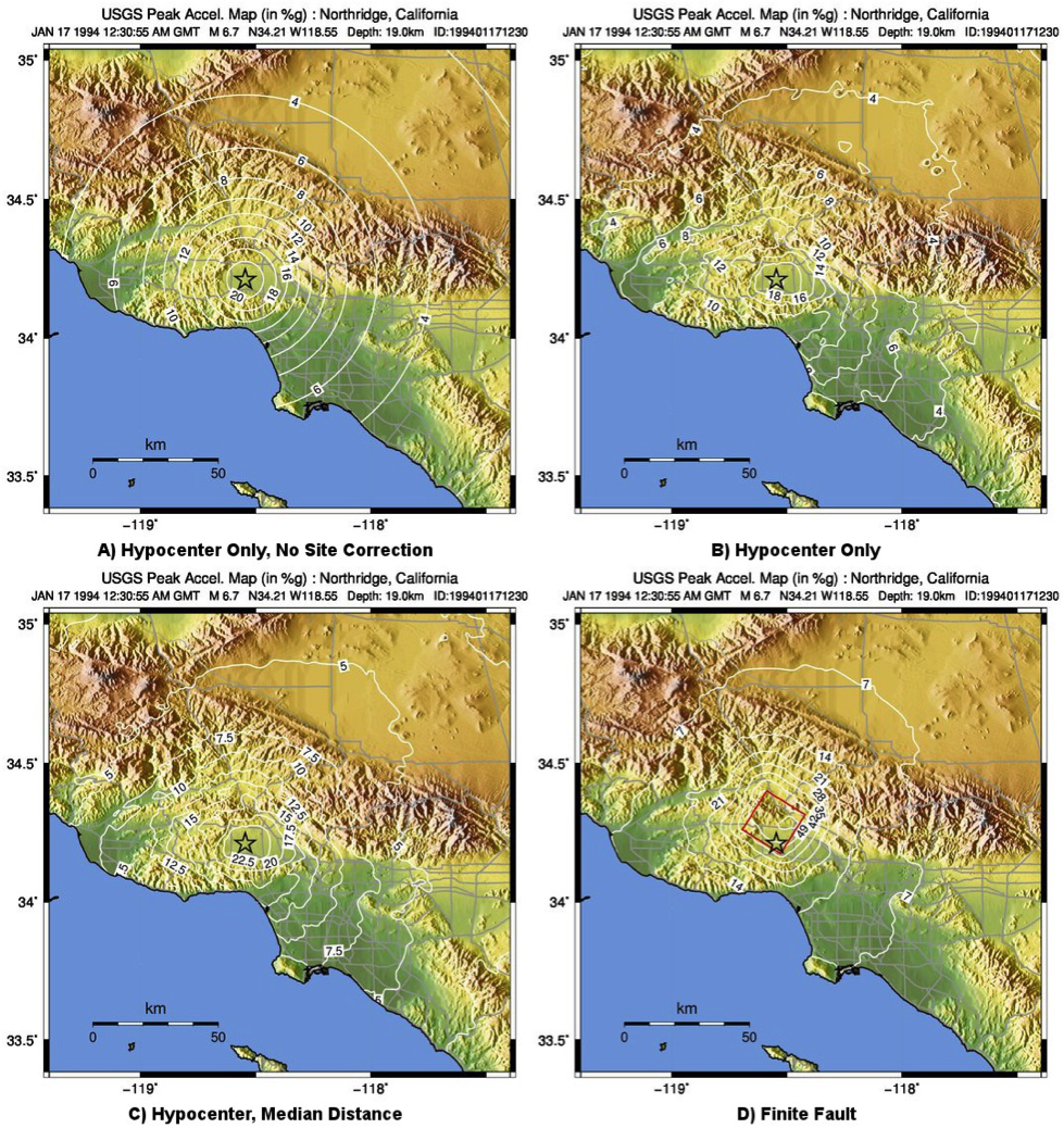
Figure 6: ShakeMap peak ground acceleration maps for the 1994 M6.7 Northridge, CA earthquake without strong motion or intensity data. A) Hypocenter only, without site amplification; B) Hypocenter, site amplification added; C) Hypocenter only, but with median distance correction added; and D) Finite fault (red rectangle) added.
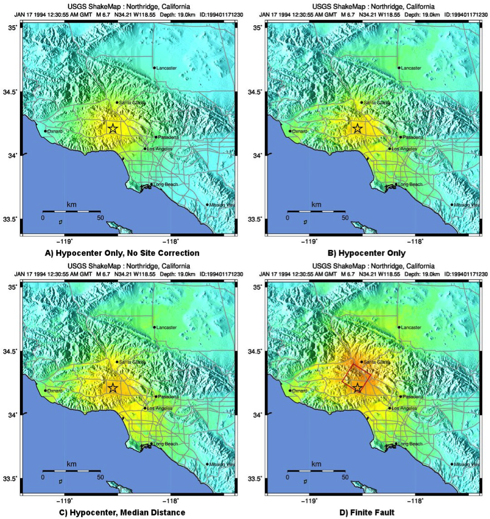
Figure 7: ShakeMap intensity maps for the 1994 M6.7 Northridge, CA earthquake without strong motion or intensity data. A) Hypocenter only, without site amplification; B) Hypocenter, site amplification added; C) Hypocenter only, but with median distance correction added; and D) Finite fault (red rectangle) added.
As the final step in correcting the observations to “rock,” if basin amplification is specified (with the -basement flag), the basin amplifications are removed from the PGM data. Currently, basin amplifications are not applied to MMI.
2.5.2. Event Bias
ShakeMap uses ground motion prediction equations (GMPEs) and, optionally, intensity prediction equations (IPEs) to supplement sparse data in its interpolation and estimation of ground motions. If sufficient data are available, we compute an event bias that effectively removes the inter-event uncertainty from the selected GMPE (IPE). This approach has been shown to greatly improve the quality of the ShakeMap ground motion estimates (for details, see Worden et al., 2012).
The bias-correction procedure is relatively straightforward: the magnitude of the earthquake is adjusted so as to minimize the misfit between the observational data and estimates at the observation points produced by the GMPE. If the user has chosen to use the directivity correction (with the -directivity flag), directivity is applied to the estimates.
In computing the total misfit, primary observations (i.e., ground-motion observations from seismic stations or MMI observations from Did You Feel It? or field surveys) are weighted as if they were GMPE predictions, whereas converted observations (i.e., primary obsertations of one type converted to another type, such as ground-motion observations converted to MMI) are down-weighted by treating them as if they were GMPE predictions converted using the GMICE (i.e., primary observations are given full weighting, whereas the converted observations are given a substantially lower weight.) Once a bias has been obtained, we flag (as outliers) any data that exceed a user- specified threshold (often three times the sigma of the GMPE at the obsertation point). The bias is then recalculated and the flagging is repeated until no outliers are found. The flagged outliers are then excluded from further processing (though the operator can choose to modify the outlier criteria or impose their inclusion).
(There are a number of configuration parameters that affect the bias computation and the flagging of outliers—see the Software Guide and grind.conf for a complete discussion of these parameters.)
The bias-adjusted GMPE is then used to create estimates for the entire output grid. If the user has opted to include directivity effects, they are applied to these estimates. See the Interpolation section for the way the GMPE-based estimates are used.
The Northridge earthquake ShakeMap provides an excellent example of the effect of bias correction. Overall, the ground motions for the Northridge earthquake exceed average estimates of existing GMPEs—in other words, it has a significant positive inter-event bias term (see Figure 8 and Figure 9, which show PGA and PGV, respectively).
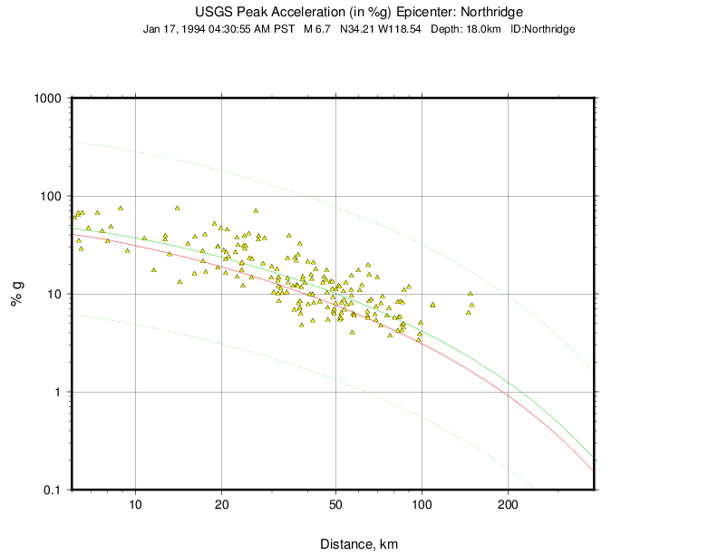
Figure 8: Plot of Northridge earthquake PGAs as a function of distance. The triangles show recorded ground motions; the red line shows the unbiased Boore and Atkinson (2008) (BA08) GMPE; the dark green lines show BA08 following the bias correction described in the text; the faint green lines show the bias-adjusted GMPE +/- three standard deviations.
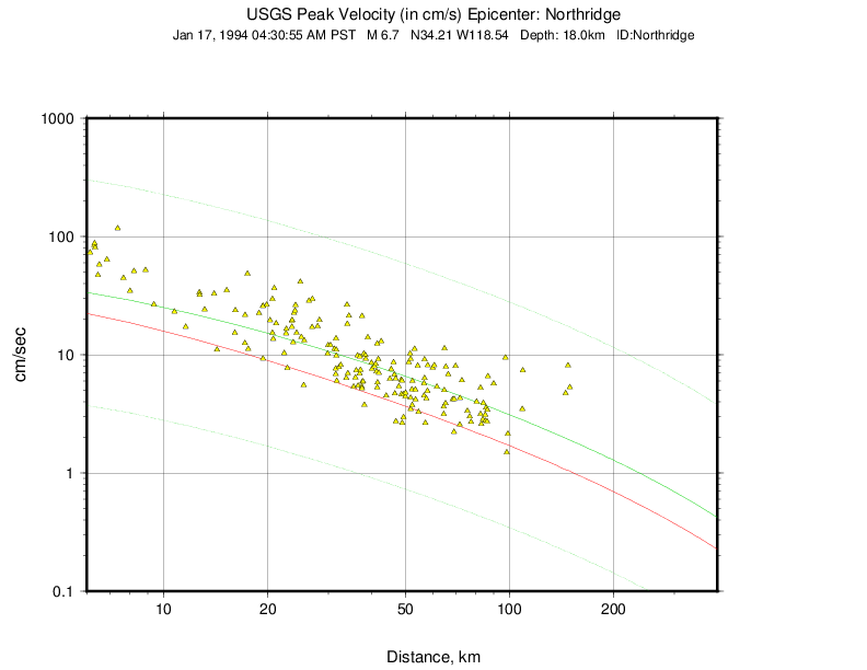
Figure 9: Plot of Northridge earthquake PGVs as a function of distance. The triangles show recorded ground motions; the red line shows the unbiased Boore and Atkinson (2008) (BA08) GMPE; the dark green lines show BA08 following the bias correction described in the text; the faint green lines show the bias-adjusted GMPE +/- three standard deviations.
The ShakeMap bias correction accommodates this behavior once a sufficient number of PGMs or intensity data are added (e.g., Figure 10 and Figure 11 A and C, show before and after bias correction, respectively). The addition of the stations provides direct shaking constraints at those locations; the bias correction additionally affects the map wherever ground motion estimates dominate (i.e., away from the stations).
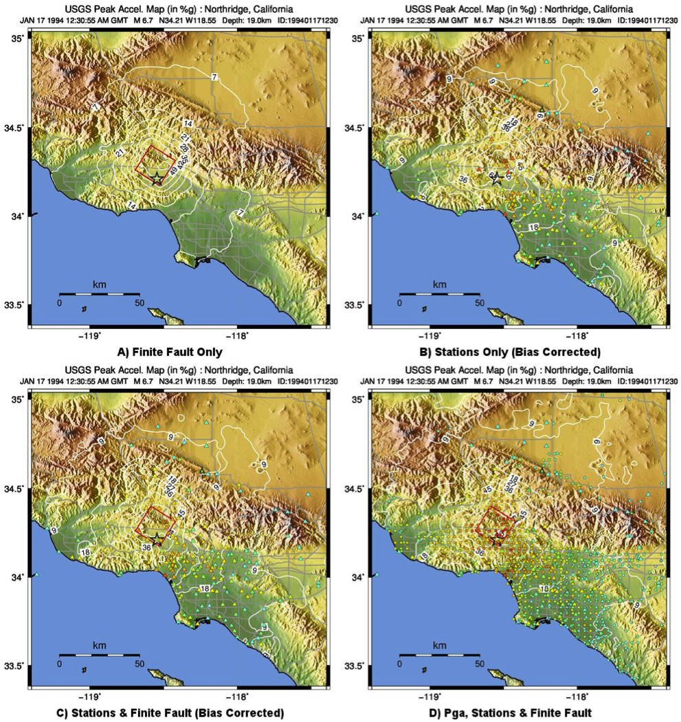
Figure 10: PGA ShakeMaps for the Northridge earthquake, showing effects of adding strong motion and intensity data. A) Finite fault only (red rectangle), no data; B) Strong motion stations (triangles) only; C) Finite Fault and strong motion stations (triangles); D) Finite Fault strong motion stations (triangles) and macroseismic data (circles). Notes: Stations and macroseismic observations are color-coded to their equivalent intensity using Worden et al. (2012).
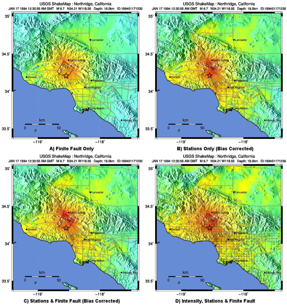
Figure 11: Intensity ShakeMaps for the Northridge earthquake, showing effects of adding strong motion and intensity data. A) Finite fault only (red rectangle), no data; B) Strong motion stations (triangles) only; C) Finite Fault and strong motion stations (triangles); D) Finite Fault strong motion stations (triangles) and macroseismic data (circles). Notes: (D) is the best possible constrained representation for this earthquake. The finite fault model without data (A) is not bias-corrected; for the Northridge earthquake, the inter-event biases are positive, indicating higher than average ground shaking for M6.7; thus, the unbiased map (A) tends to under-predict shaking shown in the data-rich, best-constrained map (D).
2.5.3. Interpolation
The interpolation procedure is described in detail in Worden et al. (2010). Here we summarize it only briefly.
To compute an estimate of ground motion at a given point in the latitude-longitude grid, ShakeMap finds an uncertainty-weighted average of 1) direct observations of ground motion or intensity, 2) direct observations of one type converted to another type (i.e., PGM converted to MMI, or vice versa), and 3) estimates from a GMPE or IPE. Note that because the output grid points are some distance from the observations, we use a spatial correlation function to obtain an uncertainty for each observation when evaluated at the outpoint point. The total uncertainty at each point is a function of the uncertainty of the direct observations obtained with the distance-to-observation uncertainty derived from the spatial correlation function, and that of the GMPE or IPE.
In the case of direct ground-motion observations, the uncertainty at the observation site is assumed to be zero, whereas at the “site” of a direct intensity observation, it is assumed to have a non-zero uncertainty due to the spatially averaged nature of intensity assignments. The uncertainty for estimates from GMPEs (and IPEs) is the stated uncertainty given in the generative publication or document. The GMPE uncertainty is often spatially constant, but this is not always the case, especially with more recent GMPEs.
For converted observations, a third uncertainty is combined with zero-distance uncertainty and the uncertainty due to spatial separation: the uncertainty associated with the conversion itself (i.e., the uncertainty of the GMICE). This additional uncertainty results in the converted observations being down-weighted in the average, relative to the primary observations.
Because a point in the output may be closer to or farther from the source than a nearby contributing observation, the observation is scaled by the ratio of the GMPE (or IPE) estimates at the output point and the observation point:
(1)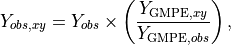
where  is the observation, and
  and
and  are the ground-motion predictions
at the observation point and the point (x,*y*), respectively. This scaling is also applied to
the converted observations with the obvious substitutions. Note that the application of
this term also accounts for any geometric terms (such as directivity or source geometry)
that the ground-motion estimates may include.
are the ground-motion predictions
at the observation point and the point (x,*y*), respectively. This scaling is also applied to
the converted observations with the obvious substitutions. Note that the application of
this term also accounts for any geometric terms (such as directivity or source geometry)
that the ground-motion estimates may include.
The formula for the estimated ground motion at a point (x,*y*) is then given by:
(2)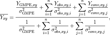
where and  are the amplitude and variance, respectively, at the point (x,*y*)
as given by the GMPE,
are the amplitude and variance, respectively, at the point (x,*y*)
as given by the GMPE,  are the observed amplitudes scaled to the point (x,*y*),
 is the variance associated with observation i at the point (x,*y*),
  are the
converted amplitudes scaled to the point (x,*y*), and
are the
converted amplitudes scaled to the point (x,*y*), and  is the variance associated
with converted observation j at the point (x,*y*).
is the variance associated
with converted observation j at the point (x,*y*).
We can then compute the estimated IM (Equation (2)) for every point in the output grid. Note that the reciprocal of the denominator of Equation (2) is the total variance at each point—a useful byproduct of the interpolation process. Again, Worden et al. (2010) provides additional details.
2.5.4. Amplify Ground Motions
At this point, ShakeMap has produced interpolated grids of ground motions (and intensities) at a site class specified as “rock.” If the operator has specified the -basement option to grind (and supplied the necessary depth-to-basement file), a basin amplification function (currently Field et al., 2000) is applied to the grids. Then, if the user has specified -qtm, site amplifications are applied to the grids, creating the final output.
2.5.5. Differences in Handling MMI
The processing of MMI is designed to be identical to the processing of PGM; however, a few differences remain:
As of this writing, there are no spatial correlation functions available for MMI. We are working on developing one, but it is not complete. We currently use the spatial correlation function for PGA as a proxy for MMI, though this approach is not optimal.
Because there are relatively few IPEs available at this time, we have introduced the idea of a virtual IPE (VIPE). If the user does not specify an IPE in grind.conf, grind will use the configured GMPE in combination with the GMICE to simulate the functionality of an IPE. In particular, the bias is computed as a magnitude adjustment to the VIPE to produce the best fit to the intensity observations (and converted observations) as described in Event Bias; and the uncertainty of the VIPE is the combined uncertainty of the GMPE and the GMICE.
As mentioned above, intensity observations are given an inherent uncertainty because of the nature of their assignment. Our research has shown that this uncertainty amounts to a few tenths of an intensity unit, but it varies with the number of responses within the averaged area. Research in this area is incomplete, and intensity data can contain both “Did You Feel It?” data and traditionally assigned intensities. Because of these considerations, we currently use a conservative value of 0.5 intensity units for the inherent uncertainty.
The directivity function we use (Rowshandel, 2010) does not have terms for intensity. This is not a problem when using the VIPE, since we can apply the directivity function to the output of the encapsulated GMPE before converting to intensity. But when a true IPE is used there is currently no explicit way to apply our directivity function. In these cases, we use the VIPE to compute two intensity grids: one with and one without directivity applied. We then subtract the former from the latter to produce a grid of directivity adjustment factors. That grid is then added to the output of the IPE. We use the same procedure when creating estimates at observation locations for computing the bias.
As mentioned above, we currently have no function for applying basin amplification to the intensity data. We hope to remedy this shortly with a solution similar to item 4, above, where we apply the basin effects through a VIPE. In practice, the main areas where basin depth models are available are also those within which station density is great (e.g., Los Angeles and San Francisco, California).
2.5.6. Fault Considerations
Small-to-moderate earthquakes can be effectively characterized as a point source, with distances being calculated from the hypocenter (or epicenter, depending on the GMPE). But accurate prediction of ground motions from larger earthquakes requires knowledge of the fault geometry. This is because ground motions attenuate with distance from the source (i.e. fault), but for a spatially extended source, that distance can be quite different from the distance to the hypocenter. Most GMPEs are developed using earthquakes with well-constrained fault geometry, and therefore are not suitable for prediction of ground motions from large earthquakes when only a point source is available. As discussed in the next section, we handle this common situation by using terms that modify the distance calculation to accommodate the unknown fault geometry. We also allow the operator to specify a finite fault, as discussed in sections Fault Dimensions and Directivity.
2.5.6.1. Median Distance and Finite Faults
As discussed in the Software Guide, the user may specify a finite fault to guide the estimates of the GMPE, but often a fault model is not available for some time following an earthquake. For larger events, this becomes problematic because the distance-to-source term ShakeMap provides to the GMPE in order to predict ground motions comes from the hypocenter (or epicenter, depending on the GMPE) rather than the actual rupture plane (or its surface projection), and for a large fault, these distances can be quite different. For a non-point source, in fact, the hypocentral distance can equal the closest distance, but it can also be significantly greater than the closest distance.
ShakeMap addresses this issue by introducing the concept of median distance. Following a study by EPRI (2003), we assume that an unknown fault of appropriate size could have any orientation, and we use EPRI’s equations to compute the distance that produces the median ground motions of all the possible fault orientations that pass through the hypocenter. (Thus, the term “median distance” is a bit of a misnomer; it is more literally “distance of median ground motion.”) Thus, for each point for which we want ground motion estimates, we compute this distance and use it as input to the GMPE. We also adjust the uncertainty of the estimate to account for the larger uncertainty associated with this situation. This feature automatically applies for earthquake magnitudes >= 5, but may be disabled with the grind flag -nomedian.
Ideally, GMPE developers would always regress not only for fault distance, but also for hypocentral distance. If this were done routinely, we would be able to initially use the hypocentral-distance regression coefficients and switch to fault-distance terms as the fault geometry was established. The median-distance approximation described above could then be discarded.
Bommer and Akkar (2012) have made the case for deriving both sets of coefficients: “The most simple, consistent, efficient and elegant solution to this problem is for all ground-motion prediction equations to be derived and presented in pairs of models, one using the analysts’ preferred extended source metric … —and another using a point- source metric, for which our preference would be hypocentral distance, Rhyp”. Indeed, Akkar et al. (2014) provide such multiple coefficients for their GMPEs for the Middle East and Europe. However, despite its utility, this strategy has not been widely adopted among the requirements for modern GMPEs (e.g., Powers et al., 2008; Abrahamson et al., 2008; 2014).
The hypocentral- or median-distance correction is not a trivial consideration. Note that for Northridge, even when the fault is unknown and there are no data, the median-distance correction (Figure 6 and Figure 7, panels B and C) brings the shaking estimates more in line with those constrained by knowledge of the fault. As mentioned earlier, the shaking for this event exhibits a positive inter-event bias term, so even with the fault location constrained, estimates still tend to under-predict the actual recordings, on average.
While the effect of this correction for the Northridge earthquake example is noticeable, for events with larger magnitudes, and thus larger rupture areas, the median-distance correction is crucial before constraints on rupture geometry are available (from finite-fault modeling, aftershock distribution, observations of surface slip, etc.) For example, in the case of the 1994 Northridge earthquake, the dimensions of the rupture are constrained from analyses of the earthquake source (e.g., Wald et al., 1996).
2.5.6.2. Fault Dimensions
The Software Guide describes the format for specifying a fault. Essentially, ShakeMap faults are one or more (connected or disconnected) planar quadrilaterals. The fault geometry is used by ShakeMap to compute fault-to-site distances for the GMPE, IPE, and GMICE, as well as to visualize the fault geometry in map view (for example, see red-line rectangles in Figure 6 and Figure 7). Examples of fault-based distances include the distance to the surface projection of the fault (for the so-called Joyner-Boore, or JB, distance), and the distance to the rupture plane.
While a finite fault is important for estimating the shaking from larger earthquakes, it is typically not necessary to develop an extremely precise fault model, or to know the rupture history that specifies the rupture propagation and slip distribution. One or two fault planes usually suffice, except for very large or complex surface-rupturing faults. In the immediate aftermath of a large earthquake, a first-order fault model based on tectonic environment, known faults, aftershock distribution, and empirical estimates based on the magnitude (e.g., Wells and Coppersmith, 1994) is often sufficient to greatly improve the ShakeMap estimates in poorly instrumented areas. In many cases, this amounts to an “educated guess”, and seismological expertise and intuition are extremely helpful. Later refinements to the faulting geometry may or may not fundamentally change the shaking pattern, depending on the density of near-source observations. As we show in a later section, dense observations greatly diminish the influence of the estimated ground motion at each grid point, obviating the need for precise fault geometries in such estimates.
2.5.6.3. Directivity
Another way in which a finite fault may affect the estimated ground motions is through directivity. Where a finite fault has been defined in ShakeMap, one may choose to apply a correction for rupture directivity. We use the approach developed by Rowshandel (2010) for the NGA GMPEs (note: caution should be exercised when applying this directivity function to non-NGA GMPEs; in addition, other directivity models give significantly different results, which is an indication that there is a high degree of uncertainty in these models). For the purposes of this calculation, we assume a constant rupture over the fault surface. While the directivity effect is secondary to fault geometry, it can make a not-insignificant difference in the near-source ground motions up-rupture or along-strike from the hypocenter.
An example of the effect of the Rowshandel (2010) directivity term is shown clearly in Figure 12 for a hypothetical strike-slip faulting scenario along the Hayward Fault in the East Bay area of San Francisco. Unilateral rupture southeastward results in stronger shaking, particularly along the southern edge of the rupture. The frequency dependence of the directivity terms provided by Rowshandel (2010) can be examined in detail by viewing the intermediate grids produced and stored in the ShakeMap output directory. In general, longer-period IMs (PGV, PSA1.0 and PSA3.0, and MMI) are more strongly affected by the directivity function employed.
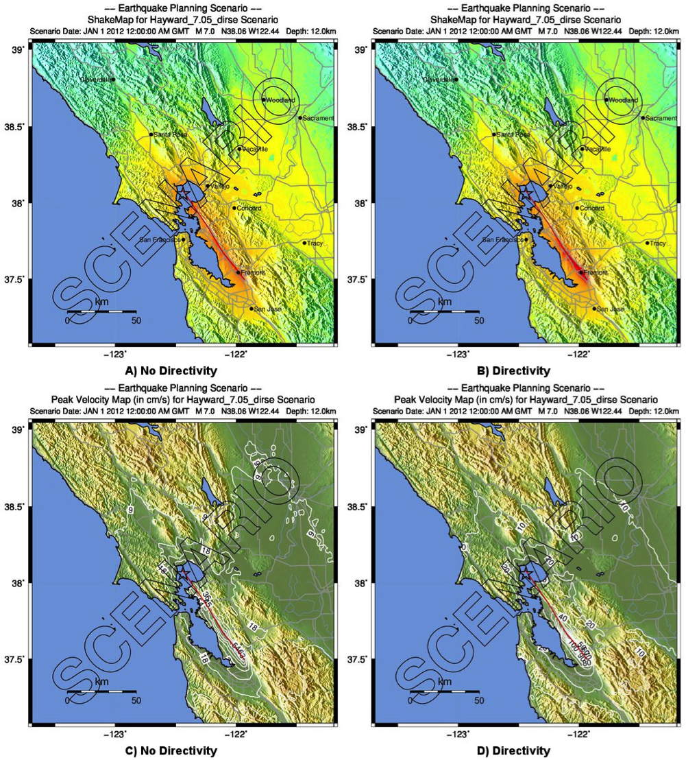
Figure 12: ShakeMap scenario intensity (top) and PGV (bottom) maps for the hypothetical M7.05 Hayward Fault, CA, earthquake: A) Intensity, No directivity; B) Intensity, Directivity added; C) PGV, No Directivity; and D) PGV, Directivity added.
2.5.7. Additional Considerations
There are a great number of details and options when running grind. Operators should familiarize themselves with grind ’s behavior by reading the Software Guide, the configuration file (grind.conf), and the program’s self-documentation (run “grind -help”). Below are a few other characteristics of grind that the operator should be familiar with.
2.5.7.1. User-supplied Estimate Grids
Much of the discussion above was centered on the use of GMPEs (and IPEs) and getting the best set of estimates from them (through bias, basin corrections, finite faults, and directivity). But the users may also supply their own grids of estimates for any or all of the ground motion parameters. ShakeMap is indifferent as to the way these estimates are generated, as long as they appear in a GMT grid in the event’s input directory, they will be used in place of the GMPE’s estimates. (See the Software Guide for the specifications of these input files.) If available, the user should also supply grids of uncertainties for the corresponding parameters—if not, ShakeMap will use the uncertainties produced by the GMPE.
User-supplied input motions allow the user to employ more sophisticated numerical ground-motion modeling techniques, ones that may include, for example, fault-slip distribution and 3D propagation effects not achievable using empirical GMPEs. The PGM output grid of such calculations can be rendered with ShakeMap, allowing users to visualize and employ familiar ShakeMap products. For instance, see the ShakeCast scenario described in Applications of ShakeMap.
2.5.7.2. Uncertainty
As mentioned above, some of the products of grind are grids of uncertainty for each parameter. This uncertainty is the result of a weighted average combination of the uncertainties of the various inputs (observations, converted observations, and estimates) at each point in the output. These gridded uncertainties are provided in the file uncertainty.xml (see Interpolated Ground Motion Grids for a description of the file format).
Because we also know the GMPE uncertainty over the grid, we can compute the ratio of the total ShakeMap uncertainty to the GMPE uncertainty. For the purposes of computing this uncertainty ratio, we use PGA as the reference IM.
Continuing with the Northridge earthquake ShakeMap example, Figure 13 presents the uncertainty maps for a variety of constraints.
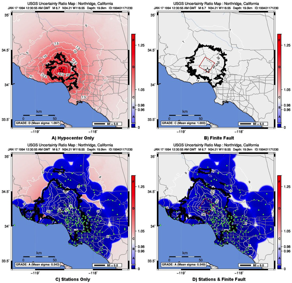
Figure 13: ShakeMap uncertainty maps for the Northridge earthquake showing effect of adding a finite fault and strong motion data. Color-coded legend shows uncertainty ratio, where ‘1.0’ indicates 1.0 times the GMPE’s sigma. A) Hypocenter (black star) only; B) Finite fault (red rectangle) added but no data (mean uncertainty is 1.00 at all locations since the site-to-source distance is constrained); C) Hypocenter and strong motion stations (triangles) only (adding stations reduces overall uncertainty); and D) Finite fault and strong motion stations. Note: Average uncertainty is computed by averaging uncertainty at grids that lie within the MMI = VI contour (bold contour line), so panel (D) is marginally higher than (C) despite added constraint (fault model). For more details see Wald et al. (2008) and Worden et al. (2010).
For a purely predictive map (of small magnitude), the uncertainty ratio will be 1.0 everywhere. For larger magnitude events, when a finite fault is not available, the ShakeMap uncertainty is greater than the nominal GMPE uncertainty (as discussed above in the section Median Distance and Finite Faults), leading to a ratio greater than 1.0 in the near-fault areas and diminishing with distance. When a finite fault is available, the ratio returns to 1.0. In areas where data are available, the ShakeMap uncertainty is less than that of the GMPE (see the section “Interpolation,” above), resulting in a ratio less than 1.0. A grid of the uncertainty ratio (and the PGA uncertainty) is provided in the output file grid.xml (see Interpolated Ground Motion Grids for a description of this file). The uncertainty ratio is the basis for the uncertainty maps and the grading system described in the User’s Guide.