ASEG to NetCDF conversion

Dataset Reference: Minsley, B.J., James, S.R., Bedrosian, P.A., Pace, M.D., Hoogenboom, B.E., and Burton, B.L., 2021, Airborne electromagnetic, magnetic, and radiometric survey of the Mississippi Alluvial Plain, November 2019 - March 2020: U.S. Geological Survey data release, https://doi.org/10.5066/P9E44CTQ.

import matplotlib.pyplot as plt
from os.path import join
from gspy import Survey

Convert the ASEG data to netcdf

# Path to example files
data_path = '..//..//supplemental//region//MAP'

# Survey Metadata file
..//supplemental = join(data_path, "data//Tempest_survey_md.json")

# Establish survey instance
survey = Survey(..//supplemental)

# Define input ASEG-format data file and associated variable mapping file
d_data = join(data_path, 'data//Tempest.dat')
d_supp = join(data_path, 'data//Tempest_data_md.json')

# Read data and format as Tabular class object
survey.add_tabular(type='aseg', data_filename=d_data, metadata_file=d_supp)

# Define input TIF-format data file and associated variable mapping file
d_grid_supp = join(data_path, 'data//Tempest_raster_md.json')
# Read data and format as Griddata class object
survey.add_raster(metadata_file = d_grid_supp)

# Define input ASEG-format model file and associated variable mapping file
m_data = join(data_path, 'model//Tempest_model.dat')
m_supp = join(data_path, 'model//Tempest_model_md.json')

# Read model data and format as Tabular class object
survey.add_tabular(type='aseg', data_filename=m_data, metadata_file=m_supp)

# Save NetCDF file
d_out = join(data_path, 'data//Tempest.nc')
survey.write_netcdf(d_out)

Read in the netcdf files

new_survey = Survey().read_netcdf(d_out)

print(new_survey.raster.magnetic_tmi)

# Once the survey is read in, we can access variables like a standard xarray dataset.

<xarray.DataArray 'magnetic_tmi' (y: 1212, x: 599)>
[725988 values with dtype=float64]
Coordinates:
    spatial_ref  float64 ...
  * x            (x) float64 2.928e+05 2.934e+05 2.94e+05 ... 6.51e+05 6.516e+05
  * y            (y) float64 1.607e+06 1.606e+06 ... 8.808e+05 8.802e+05
Attributes:
    standard_name:  total_magnetic_intensity
    null_value:     -9999.99
    units:          nT
    valid_range:    [-17504.6640625   11490.32324219]
    long_name:      Total magnetic intensity, diurnally corrected and filtered

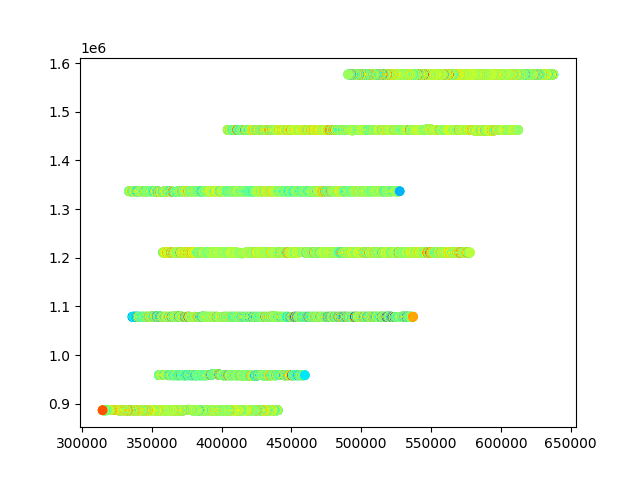
Plotting

plt.figure()
new_survey.tabular[0].gs_tabular.scatter('X_PrimaryField', cmap='jet')

# plt.figure()
# new_survey.raster.gs_raster.pcolor('magnetic_tmi', vmin=-1000, vmax=1000, cmap='jet')

# plt.figure()
# new_survey.tabular[1].gs_tabular.scatter('PhiD')

# print(new_survey.tabular[0])
# print(new_survey.tabular[0]['x'].attrs)
# print(new_survey.tabular[0]['EMX_HPRG'])

plt.show()