ASEG to NetCDF

This example demonstrates the workflow for creating a GS file from the ASEG file format, as well as how to add multiple associated datasets to the Survey (e.g., Tabular and Raster groups). Specifically, this AEM survey contains the following datasets:

Raw AEM data, from the Tempest system
Inverted resistivity models
An interpolated map of total magnetic intensity

Dataset Reference: Minsley, B.J., James, S.R., Bedrosian, P.A., Pace, M.D., Hoogenboom, B.E., and Burton, B.L., 2021, Airborne electromagnetic, magnetic, and radiometric survey of the Mississippi Alluvial Plain, November 2019 - March 2020: U.S. Geological Survey data release, https://doi.org/10.5066/P9E44CTQ.

import matplotlib.pyplot as plt
from os.path import join
import gspy

Convert the ASEG data to NetCDF

Initialize the Survey

# Path to example files
data_path = '..//..//..//..//example_material//example_2'

# Survey Metadata file
metadata = join(data_path, "data//Tempest_survey_md.yml")

# Establish survey instance
survey = gspy.Survey.from_dict(metadata)

Raw Data -

data_container = survey.gs.add_container('data', **dict(content = "raw and processed data"))

# Import raw AEM data from ASEG-format.
# Define input data file and associated metadata file
d_data = join(data_path, 'data//Tempest.dat')
d_supp = join(data_path, 'data//Tempest_data_md.yml')

# Add the raw AEM data as a tabular dataset
rd = data_container.gs.add(key='raw_data', data_filename=d_data, metadata_file=d_supp)

Inverted Models

model_container = survey.gs.add_container('models', **dict(content = "inverted models"))

# Import inverted AEM models from ASEG-format.
# Define input data file and associated metadata file
m_data = join(data_path, 'model//Tempest_model.dat')
m_supp = join(data_path, 'model//Tempest_model_md.yml')

# Read model data and format as Tabular class object
model_container.gs.add(key='inverted_models', data_filename=m_data, metadata_file=m_supp)

<xarray.DatasetView> Size: 31MB
Dimensions:                  (index: 20701, layer_depth: 30, nv: 2,
                              gate_times: 15)
Coordinates:
    spatial_ref              float64 8B 0.0
  * index                    (index) int32 83kB 0 1 2 3 ... 20698 20699 20700
  * layer_depth              (layer_depth) float64 240B 1.5 4.65 ... 424.2 467.5
  * nv                       (nv) int64 16B 0 1
  * gate_times               (gate_times) float64 120B 1.085e-05 ... 0.01338
    x                        (index) float64 166kB 3.579e+05 ... 4.906e+05
    y                        (index) float64 166kB 1.211e+06 ... 1.577e+06
    z                        (index) float64 166kB 45.83 46.61 ... 179.4 177.2
Data variables: (12/49)
    layer_depth_bnds         (layer_depth, nv) float64 480B 0.0 3.0 ... 489.1
    gate_times_bnds          (gate_times, nv) float64 240B 5.43e-06 ... 0.01666
    uniqueid                 (index) int32 83kB 0 1 2 3 ... 20698 20699 20700
    survey                   (index) int32 83kB 9999 9999 9999 ... 9999 9999
    date                     (index) int32 83kB 20191128 20191128 ... 20200227
    flight                   (index) int32 83kB 10 10 10 10 10 ... 70 70 70 70
    ...                       ...
    phic                     (index) float64 166kB 0.4491 0.4759 ... 1.61 1.289
    phit                     (index) float64 166kB 0.0 0.0 0.0 ... 0.0 0.0 0.0
    phig                     (index) float64 166kB 0.9652 0.6608 ... 1.457
    phis                     (index) float64 166kB 0.1158 0.1392 ... 0.1705
    lambda                   (index) float64 166kB 0.5968 0.5487 ... 1.771
    iterations               (index) int32 83kB 20 19 25 25 25 ... 30 30 27 29
Attributes:
    content:  inverted resistivity models
    comment:  This dataset includes inverted resistivity models derived from ...

Magnetic Intensity Map

data_derived = data_container.gs.add_container('derived_maps', **dict(content = "derived maps"))

# Import the magnetic data from TIF-format.
# Define input metadata file (which contains the TIF filenames linked with desired variable names)
r_supp = join(data_path, 'data//Tempest_raster_md.yml')

# Read data and format as Raster class object
data_derived.gs.add(key='maps', metadata_file = r_supp)

# Save NetCDF file
d_out = join(data_path, 'data//Tempest.nc')
survey.gs.to_netcdf(d_out)

Read back in the NetCDF file

new_survey = gspy.open_datatree(d_out)['survey']

# Once the survey is read in, we can access variables like a standard xarray dataset.
print(new_survey['data/derived_maps/maps'].magnetic_tmi)
print(new_survey['data/derived_maps/maps']['magnetic_tmi'])

<xarray.DataArray 'magnetic_tmi' (y: 1212, x: 599)> Size: 6MB
[725988 values with dtype=float64]
Coordinates:
    spatial_ref  float64 8B ...
  * x            (x) float64 5kB 2.928e+05 2.934e+05 ... 6.51e+05 6.516e+05
  * y            (y) float64 10kB 1.607e+06 1.606e+06 ... 8.808e+05 8.802e+05
Attributes:
    standard_name:  total_magnetic_intensity
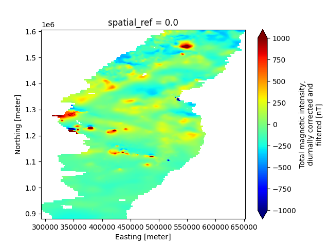
    long_name:      Total magnetic intensity, diurnally corrected and filtered
    units:          nT
    null_value:     1.70141e+38
    valid_range:    [-17504.6640625   11490.32324219]
    grid_mapping:   spatial_ref
<xarray.DataArray 'magnetic_tmi' (y: 1212, x: 599)> Size: 6MB
[725988 values with dtype=float64]
Coordinates:
    spatial_ref  float64 8B ...
  * x            (x) float64 5kB 2.928e+05 2.934e+05 ... 6.51e+05 6.516e+05
  * y            (y) float64 10kB 1.607e+06 1.606e+06 ... 8.808e+05 8.802e+05
Attributes:
    standard_name:  total_magnetic_intensity
    long_name:      Total magnetic intensity, diurnally corrected and filtered
    units:          nT
    null_value:     1.70141e+38
    valid_range:    [-17504.6640625   11490.32324219]
    grid_mapping:   spatial_ref

Plotting

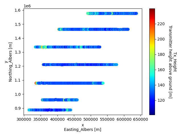
# Make a scatter plot of a specific tabular variable, using GSPy's plotter
plt.figure()
new_survey['data']['raw_data'].gs.scatter(x='x', hue='tx_height', cmap='jet')

# Make a 2-D map plot of a specific raster variable, using Xarrays's plotter
plt.figure()
new_survey['data/derived_maps/maps']['magnetic_tmi'].plot(cmap='jet', robust=True)
plt.show()

Total running time of the script: (0 minutes 9.086 seconds)

Gallery generated by Sphinx-Gallery