CSV to NetCDF

This example demonstrates how to convert comma-separated values (CSV) data to the GS NetCDF format. Specifically this example includes:

Raw AEM data, from the Resolve system
Inverted resistivity models

Dataset Reference: Burton, B.L., Minsley, B.J., Bloss, B.R., and Kress, W.H., 2021, Airborne electromagnetic, magnetic, and radiometric survey of the Mississippi Alluvial Plain, November 2018 - February 2019: U.S. Geological Survey data release, https://doi.org/10.5066/P9XBBBUU.

import matplotlib.pyplot as plt
from os.path import join
import gspy

Convert the resolve csv data to NetCDF

Initialize the Survey

# Path to example files
data_path = '..//..//..//..//example_material//example_2'

# Survey metadata file
metadata = join(data_path, "data//Resolve_survey_md.yml")
# Establish the Survey
survey = gspy.Survey.from_dict(metadata)

Import raw AEM data from CSV-format.

data_container = survey.gs.add_container('data', **dict(content = "raw and processed data"))

# Define input data file and associated metadata file
d_data = join(data_path, 'data//Resolve.csv')
d_supp = join(data_path, 'data//Resolve_data_md.yml')

# Add the raw AEM data as a tabular dataset
data_container.gs.add(key='raw_data', data_filename=d_data, metadata_file=d_supp)

<xarray.DatasetView> Size: 12MB
Dimensions:           (index: 2334, layer_depth: 31, nv: 2, spec_sample: 256,
                       frequency: 6)
Coordinates:
    spatial_ref       float64 8B 0.0
  * index             (index) int32 9kB 0 1 2 3 4 5 ... 2329 2330 2331 2332 2333
  * layer_depth       (layer_depth) float64 248B 2.5 7.5 12.5 ... 147.5 152.5
  * nv                (nv) int64 16B 0 1
    x                 (index) float64 19kB 5.351e+05 5.341e+05 ... 5.315e+05
    y                 (index) float64 19kB 1.205e+06 1.205e+06 ... 1.205e+06
    z                 (index) float64 19kB 42.82 43.96 42.74 ... 42.73 43.3
  * spec_sample       (spec_sample) int64 2kB 0 1 2 3 4 ... 251 252 253 254 255
  * frequency         (frequency) int64 48B 400 1800 3300 8200 40000 140000
Data variables: (12/79)
    layer_depth_bnds  (layer_depth, nv) float64 496B 0.0 5.0 5.0 ... 150.0 155.0
    line              (index) int32 9kB 10010 10010 10010 ... 19020 19020 19020
    date              (index) int64 19kB 20180302 20180302 ... 20180226 20180226
    utc_time          (index) float64 19kB 1.92e+05 1.92e+05 ... 1.741e+05
    flight            (index) int64 19kB 28022 28022 28022 ... 28011 28011 28011
    fiducial          (index) float64 19kB 969.8 999.8 ... 2.49e+03 2.52e+03
    ...                ...
    ip_filtered       (index, frequency) float64 112kB 118.0 302.9 ... 2.008e+03
    qd_filtered       (index, frequency) float64 112kB 169.5 423.8 ... 695.7
    ip_pgadj          (index, frequency) float64 112kB 118.0 302.9 ... 2.008e+03
    qd_pgadj          (index, frequency) float64 112kB 169.5 423.8 ... 695.7
    ip_final          (index, frequency) float64 112kB 118.5 302.9 ... 2.008e+03
    qd_final          (index, frequency) float64 112kB 169.3 423.8 ... 696.3
Attributes:
    content:     raw data
    comment:     This dataset includes minimally processed (raw) AEM data
    type:        data
    method:      electromagnetic
    instrument:  resolve

Import inverted AEM models from CSV-format.

model_container = survey.gs.add_container('models', **dict(content = "inverted models"))

# Define input model file and associated metadata file
m_data = join(data_path, 'model//Resolve_model.csv')
m_supp = join(data_path, 'model//Resolve_model_md.yml')

# Add the inverted AEM models as a tabular dataset
model_container.gs.add(key="model", data_filename=m_data, metadata_file=m_supp)

Save to NetCDF file

d_out = join(data_path, 'model//Resolve.nc')
survey.gs.to_netcdf(d_out)

Reading back in the GS NetCDF file

new_survey = gspy.open_datatree(d_out)['survey']

# Check the Survey information

Plotting

# Make a scatter plot of a specific data variable, using GSPy's plotter
plt.figure()
new_survey['data/raw_data'].gs.scatter(hue='dtm', vmin=30, vmax=50)

# Subsetting by line number, and plotting by distance along that line
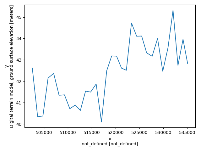
tmp = new_survey['data/raw_data'].gs.subset('line', 10010)
# tmp = new_survey['data'].where(new_survey['data'].dataset['line']==10010)
plt.figure()
# plt.subplot(121)
# tmp.gs_tabular.plot(hue='DTM')
# plt.subplot(122)
# tmp.gs_tabular.scatter(x='x', y='DTM')
tmp.gs.scatter(y='dtm')

#IF YOU SPECIFY HUE ITS A 2D COLOUR Plot
#OTHERWISE ITS JUST A PLOT (LINE POINTS ETC)

# Make a scatter plot of a specific model variable, using GSPy's plotter
plt.figure()
new_survey['models/model'].gs.scatter(hue='doi_standard')
plt.show()

Total running time of the script: (0 minutes 4.024 seconds)

Gallery generated by Sphinx-Gallery