Multi-dataset Survey

This example demonstrates the typical workflow for creating a GS file for an AEM survey in its entirety, i.e., the NetCDF file contains all related datasets together, e.g., raw data, processed data, inverted models, and derivative products. Specifically, this survey contains:

Minimally processed (raw) AEM data and raw/processed magnetic data provided by SkyTEM
Fully processed AEM data used as input to inversion
Laterally constrained inverted resistivity models
Point-data estimates of bedrock depth derived from the AEM models
Interpolated magnetic and bedrock depth grids

Note: To make the size of this example more managable, some of the input datasets have been downsampled relative to the source files in the data release referenced below.

Dataset Reference: Minsley, B.J, Bloss, B.R., Hart, D.J., Fitzpatrick, W., Muldoon, M.A., Stewart, E.K., Hunt, R.J., James, S.R., Foks, N.L., and Komiskey, M.J., 2022, Airborne electromagnetic and magnetic survey data, northeast Wisconsin (ver. 1.1, June 2022): U.S. Geological Survey data release, https://doi.org/10.5066/P93SY9LI.

import matplotlib.pyplot as plt
from os.path import join
import numpy as np
import gspy

Convert the Skytem csv data to NetCDF

Initialize the Survey

# Path to example files
data_path = '..//..//..//..//example_material//example_3'

# Survey metadata file
metadata = join(data_path, "data//LoupeEM_survey_md.yml")

# Establish the Survey
survey = gspy.Survey.from_dict(metadata)

data_container = survey.gs.add_container('data')

data = join(data_path, 'data//Kankakee.dat')
metadata = join(data_path, 'data//Loupe_data_metadata.yml')
data_container.gs.add(key='raw_data', data_filename=data, metadata_file=metadata)

<xarray.DatasetView> Size: 11MB
Dimensions:       (index: 11633, gate_times: 23)
Coordinates:
    spatial_ref   float64 8B 0.0
  * index         (index) int32 47kB 0 1 2 3 4 ... 11628 11629 11630 11631 11632
    x             (index) float64 93kB 5.248e+05 5.248e+05 ... 5.248e+05
    y             (index) float64 93kB 4.583e+06 4.583e+06 ... 4.583e+06
    z             (index) float64 93kB 211.5 211.5 211.5 ... 204.4 204.4 204.4
  * gate_times    (gate_times) float64 184B 1.297e-05 1.495e-05 ... 0.002183
Data variables: (12/45)
    fid           (index) object 93kB '1' '2' '3' ... '12120' '12121' '12122'
    acq           (index) float64 93kB 1.0 1.0 1.0 1.0 ... 25.0 25.0 25.0 25.0
    acq_rdg       (index) float64 93kB 0.0 1.0 2.0 3.0 ... 364.0 365.0 366.0
    acq_time      (index) object 93kB '20230808T175252.504075397Z' ... '20230...
    time          (index) object 93kB '20230808T175253.000000000Z' ... '20230...
    ts            (index) float64 93kB 1.692e+09 1.692e+09 ... 1.692e+09
    ...            ...
    y_powerphase  (index) float64 93kB 1.006 1.07 1.008 ... -2.935 -2.884 -2.952
    z_powerphase  (index) float64 93kB 1.663 1.679 1.748 ... 0.9777 1.006 1.041
    X_CH          (index, gate_times) float64 2MB 491.5 357.4 ... 0.01459
    Y_CH          (index, gate_times) float64 2MB -6.219 6.26 ... -0.002063
    Z_CH          (index, gate_times) float64 2MB 499.8 434.7 ... 6.37e-05
    line          (index) int64 93kB 1 1 1 1 1 1 1 1 ... 25 25 25 25 25 25 25 25
Attributes:
    content:     raw data
    comment:     This dataset includes minimally processed (raw) AEM data
    type:        data
    method:      electromagnetic
    instrument:  loupe

xarray.DataTree

Groups: (1)
<xarray.DatasetView> Size: 48kB Dimensions: (index: 11633, gate_times: 23, nv: 2, n_transmitters: 1, z_waveform_time: 4, z_loop_vertices: 8, xyz: 3, n_receivers: 3, n_components: 3) Coordinates: * index (index) int32 47kB 0 1 ... 11631 11632 * gate_times (gate_times) float64 184B 1.297e-05 ... * nv (nv) int64 16B 0 1 * n_transmitters (n_transmitters) int64 8B 0 * z_waveform_time (z_waveform_time) float64 32B -0.002... * xyz (xyz) int64 24B 0 1 2 * z_loop_vertices (z_loop_vertices) float64 64B 0.0 ..... * n_receivers (n_receivers) int64 24B 0 1 2 * n_components (n_components) int64 24B 0 1 2 Data variables: (12/25) gate_times_bnds (gate_times, nv) float64 368B 1.098e... transmitter_label (n_transmitters) <U1 4B 'z' transmitter_area (n_transmitters) float64 8B 0.358 transmitter_base_frequency (n_transmitters) float64 8B 90.0 transmitter_current_scale_factor (n_transmitters) float64 8B 1.0 transmitter_number_of_turns (n_transmitters) int32 4B 13 ... ... component_receivers (n_components) <U1 12B 'x' 'y' 'z' component_sample_rate (n_components) float64 24B 1.0 1.0 1.0 component_txrx_dx (n_components) float64 24B -10.0 ...... component_txrx_dy (n_components) float64 24B 0.0 0.0 0.0 component_txrx_dz (n_components) float64 24B -0.75 ...... component_gate_times (n_components) <U10 120B 'gate_times... Attributes: type: system mode: ground method: electromagnetic submethod: time domain instrument: loupe
loupe_system
Groups: (0)
Dimensions:
index: 11633
gate_times: 23
nv: 2
n_transmitters: 1
z_waveform_time: 4
z_loop_vertices: 8
xyz: 3
n_receivers: 3
n_components: 3
Coordinates: (7)
nv
(nv)
int64
0 1
standard_name :
nv
long_name :
Number of vertices for bounding variables
units :
not_defined
null_value :
not_defined
valid_range :
[0 1]
grid_mapping :
spatial_ref
axis :
NV
array([0, 1])
n_transmitters
(n_transmitters)
int64
0
standard_name :
n_transmitters
long_name :
Number of transmitter loops in this system
units :
not_defined
null_value :
not_defined
valid_range :
[0 0]
grid_mapping :
spatial_ref
axis :
N_TRANSMITTERS
array([0])
z_waveform_time
(z_waveform_time)
float64
-0.002778 -0.002769 0.0 9e-06
standard_name :
z_waveform_time
long_name :
z waveform time
units :
s
null_value :
not_defined
valid_range :
[-2.77778e-03 9.00000e-06]
grid_mapping :
spatial_ref
axis :
Z_WAVEFORM_TIME
array([-2.77778e-03, -2.76878e-03, 0.00000e+00, 9.00000e-06])
xyz
(xyz)
int64
0 1 2
standard_name :
xyz
long_name :
spatial dimensions of the loop vertices
units :
m
null_value :
not_defined
valid_range :
[0 2]
grid_mapping :
spatial_ref
axis :
XYZ
array([0, 1, 2])
z_loop_vertices
(z_loop_vertices)
float64
0.0 1.0 2.0 3.0 4.0 5.0 6.0 7.0
standard_name :
z_loop_vertices
long_name :
loop vertices
units :
not_defined
null_value :
not_defined
valid_range :
[0. 7.]
grid_mapping :
spatial_ref
axis :
Z_LOOP_VERTICES
array([0., 1., 2., 3., 4., 5., 6., 7.])
n_receivers
(n_receivers)
int64
0 1 2
standard_name :
n_receivers
long_name :
Number of receiver loops in this system
units :
not_defined
null_value :
not_defined
valid_range :
[0 2]
grid_mapping :
spatial_ref
axis :
N_RECEIVERS
array([0, 1, 2])
n_components
(n_components)
int64
0 1 2
standard_name :
n_components
long_name :
transmitter for each component
units :
not_defined
null_value :
not_defined
valid_range :
[0 2]
grid_mapping :
spatial_ref
axis :
N_COMPONENTS
array([0, 1, 2])
Data variables: (25)
gate_times_bnds
(gate_times, nv)
float64
1.098e-05 1.495e-05 ... 0.002557
standard_name :
gate_times_bounds
long_name :
receiver gate times cell boundaries
units :
seconds
null_value :
not_defined
valid_range :
[1.09800e-05 2.55662e-03]
grid_mapping :
spatial_ref
array([[1.09800e-05, 1.49500e-05], [1.29700e-05, 1.69400e-05], [1.49500e-05, 1.89200e-05], [1.69400e-05, 2.09000e-05], [1.89200e-05, 2.28900e-05], [2.09000e-05, 2.88400e-05], [2.68600e-05, 3.47900e-05], [3.28100e-05, 4.47100e-05], [4.07500e-05, 5.66200e-05], [5.26500e-05, 7.24900e-05], [6.65400e-05, 9.03500e-05], [8.63800e-05, 1.18130e-04], [1.12170e-04, 1.55830e-04], [1.45900e-04, 2.01460e-04], [1.91540e-04, 2.66940e-04], [2.53050e-04, 3.52250e-04], [3.32410e-04, 4.67330e-04], [4.39560e-04, 6.22100e-04], [5.82410e-04, 8.22490e-04], [7.72890e-04, 1.09233e-03], [1.02487e-03, 1.44948e-03], [1.36019e-03, 1.92567e-03], [1.80860e-03, 2.55662e-03]])
transmitter_label
(n_transmitters)
<U1
'z'
standard_name :
transmitter label
long_name :
Label of the transmitter
units :
not_defined
null_value :
not_defined
grid_mapping :
spatial_ref
array(['z'], dtype='<U1')
transmitter_area
(n_transmitters)
float64
0.358
standard_name :
transmitter area
long_name :
Loop area of the transmitter
units :
m^{2}
null_value :
not_defined
valid_range :
[0.358 0.358]
grid_mapping :
spatial_ref
array([0.358])
transmitter_base_frequency
(n_transmitters)
float64
90.0
standard_name :
transmitter base frequency
long_name :
Base frequency of the transmitter
units :
Hz
null_value :
not_defined
valid_range :
[90. 90.]
grid_mapping :
spatial_ref
array([90.])
transmitter_current_scale_factor
(n_transmitters)
float64
1.0
standard_name :
transmitter current scale factor
long_name :
Current scale factor of the transmitter
units :
not_defined
null_value :
not_defined
valid_range :
[1. 1.]
grid_mapping :
spatial_ref
array([1.])
transmitter_number_of_turns
(n_transmitters)
int32
13
standard_name :
number_of_transmitter_turns
long_name :
Number of loops turns of the transmitter
units :
not_defined
null_value :
not_defined
valid_range :
[13 13]
grid_mapping :
spatial_ref
array([13], dtype=int32)
transmitter_on_time
(n_transmitters)
float64
0.002769
standard_name :
transmitter_on_time
long_name :
On time of the transmitter
units :
s
null_value :
not_defined
valid_range :
[0.00276878 0.00276878]
grid_mapping :
spatial_ref
array([0.00276878])
transmitter_off_time
(n_transmitters)
float64
0.002787
standard_name :
transmitter_off_time
long_name :
Off time of the transmitter
units :
s
null_value :
not_defined
valid_range :
[0.00278678 0.00278678]
grid_mapping :
spatial_ref
array([0.00278678])
transmitter_orientation
(n_transmitters)
<U1
'z'
standard_name :
transmitter_orientation
long_name :
Orientation of the transmitter loop
units :
not_defined
null_value :
not_defined
grid_mapping :
spatial_ref
array(['z'], dtype='<U1')
transmitter_peak_current
(n_transmitters)
float64
20.0
standard_name :
transmitter_peak_current
long_name :
Peak current of the transmitter
units :
A
null_value :
not_defined
valid_range :
[20. 20.]
grid_mapping :
spatial_ref
array([20.])
transmitter_waveform_type
(n_transmitters)
<U9
'trapezoid'
standard_name :
transmitter_waveform_type
long_name :
Waveform type of the transmitter
units :
not_defined
null_value :
not_defined
grid_mapping :
spatial_ref
array(['trapezoid'], dtype='<U9')
z_waveform_current
(z_waveform_time)
float64
0.0 1.0 1.0 0.0
standard_name :
z_waveform_current
long_name :
z waveform current
units :
A
null_value :
not_defined
valid_range :
[0. 1.]
grid_mapping :
spatial_ref
array([0., 1., 1., 0.])
z_loop_coordinates
(z_loop_vertices, xyz)
float64
0.33 0.14 0.0 ... 0.33 -0.14 0.0
standard_name :
z_loop_coordinates
long_name :
z loop coordinates
units :
m
null_value :
not_defined
valid_range :
[-0.33 0.33]
grid_mapping :
spatial_ref
array([[ 0.33, 0.14, 0. ], [ 0.14, 0.33, 0. ], [-0.14, 0.33, 0. ], [-0.33, 0.14, 0. ], [-0.33, -0.14, 0. ], [-0.14, -0.33, 0. ], [ 0.14, -0.33, 0. ], [ 0.33, -0.14, 0. ]])
receiver_label
(n_receivers)
<U1
'x' 'y' 'z'
standard_name :
receiver label
long_name :
Label of the receiver
units :
not_defined
null_value :
not_defined
grid_mapping :
spatial_ref
array(['x', 'y', 'z'], dtype='<U1')
receiver_coil_low_pass_filter
(n_receivers)
float64
1e+05 1e+05 1e+05
standard_name :
receiver_coil_low_pass_filter
long_name :
Low pass filter frequencey of the coil
units :
Hz
null_value :
not_defined
valid_range :
[100000. 100000.]
grid_mapping :
spatial_ref
array([100000., 100000., 100000.])
receiver_orientation
(n_receivers)
<U1
'x' 'y' 'z'
standard_name :
receiver_orientation
long_name :
Orientation of the receiver loop
units :
not_defined
null_value :
not_defined
grid_mapping :
spatial_ref
array(['x', 'y', 'z'], dtype='<U1')
receiver_instrument_low_pass_filter
(n_receivers)
float64
2.5e+05 2.5e+05 2.5e+05
standard_name :
receiver_instrument_low_pass_filter
long_name :
Low pass filter frequency of the instrument
units :
Hz
null_value :
not_defined
valid_range :
[250000. 250000.]
grid_mapping :
spatial_ref
array([250000., 250000., 250000.])
receiver_area
(n_receivers)
float64
200.0 200.0 200.0
standard_name :
receiver_area
long_name :
Area of the receiver loop
units :
m^{2}
null_value :
not_defined
valid_range :
[200. 200.]
grid_mapping :
spatial_ref
array([200., 200., 200.])
component_transmitters
(n_components)
<U1
'z' 'z' 'z'
standard_name :
component_transmitters
long_name :
Transmitter for each component
units :
not_defined
null_value :
not_defined
grid_mapping :
spatial_ref
array(['z', 'z', 'z'], dtype='<U1')
component_receivers
(n_components)
<U1
'x' 'y' 'z'
standard_name :
component_receivers
long_name :
Receiver for each component
units :
not_defined
null_value :
not_defined
grid_mapping :
spatial_ref
array(['x', 'y', 'z'], dtype='<U1')
component_sample_rate
(n_components)
float64
1.0 1.0 1.0
standard_name :
component_sample_rate
long_name :
Sampling rate of this component
units :
s
null_value :
not_defined
valid_range :
[1. 1.]
grid_mapping :
spatial_ref
array([1., 1., 1.])
component_txrx_dx
(n_components)
float64
-10.0 -10.0 -10.0
standard_name :
component_txrx_dx
long_name :
x offset for each transmitter receiver pair
units :
m
null_value :
not_defined
valid_range :
[-10. -10.]
grid_mapping :
spatial_ref
array([-10., -10., -10.])
component_txrx_dy
(n_components)
float64
0.0 0.0 0.0
standard_name :
component_txrx_dy
long_name :
y offset for each transmitter receiver pair
units :
m
null_value :
not_defined
valid_range :
[0. 0.]
grid_mapping :
spatial_ref
array([0., 0., 0.])
component_txrx_dz
(n_components)
float64
-0.75 -0.75 -0.75
standard_name :
component_txrx_dz
long_name :
vertical offset for each transmitter receiver pair
units :
m
null_value :
not_defined
valid_range :
[-0.75 -0.75]
grid_mapping :
spatial_ref
array([-0.75, -0.75, -0.75])
component_gate_times
(n_components)
<U10
'gate_times' ... 'gate_times'
standard_name :
component_gate_times
long_name :
Gate times for this component
units :
s
null_value :
not_defined
grid_mapping :
spatial_ref
array(['gate_times', 'gate_times', 'gate_times'], dtype='<U10')
Attributes: (5)
type :
system
mode :
ground
method :
electromagnetic
submethod :
time domain
instrument :
loupe
Dimensions:
- index: 11633
- gate_times: 23
Coordinates: (6)
- spatial_ref
  ()
  float64
  0.0
  crs_wkt :
  PROJCRS["WGS 84 / UTM zone 16N",BASEGEOGCRS["WGS 84",ENSEMBLE["World Geodetic System 1984 ensemble",MEMBER["World Geodetic System 1984 (Transit)"],MEMBER["World Geodetic System 1984 (G730)"],MEMBER["World Geodetic System 1984 (G873)"],MEMBER["World Geodetic System 1984 (G1150)"],MEMBER["World Geodetic System 1984 (G1674)"],MEMBER["World Geodetic System 1984 (G1762)"],MEMBER["World Geodetic System 1984 (G2139)"],MEMBER["World Geodetic System 1984 (G2296)"],ELLIPSOID["WGS 84",6378137,298.257223563,LENGTHUNIT["metre",1]],ENSEMBLEACCURACY[2.0]],PRIMEM["Greenwich",0,ANGLEUNIT["degree",0.0174532925199433]],ID["EPSG",4326]],CONVERSION["UTM zone 16N",METHOD["Transverse Mercator",ID["EPSG",9807]],PARAMETER["Latitude of natural origin",0,ANGLEUNIT["degree",0.0174532925199433],ID["EPSG",8801]],PARAMETER["Longitude of natural origin",-87,ANGLEUNIT["degree",0.0174532925199433],ID["EPSG",8802]],PARAMETER["Scale factor at natural origin",0.9996,SCALEUNIT["unity",1],ID["EPSG",8805]],PARAMETER["False easting",500000,LENGTHUNIT["metre",1],ID["EPSG",8806]],PARAMETER["False northing",0,LENGTHUNIT["metre",1],ID["EPSG",8807]]],CS[Cartesian,2],AXIS["(E)",east,ORDER[1],LENGTHUNIT["metre",1]],AXIS["(N)",north,ORDER[2],LENGTHUNIT["metre",1]],USAGE[SCOPE["Navigation and medium accuracy spatial referencing."],AREA["Between 90°W and 84°W, northern hemisphere between equator and 84°N, onshore and offshore. Belize. Canada - Manitoba; Nunavut; Ontario. Costa Rica. Cuba. Ecuador - Galapagos. El Salvador. Guatemala. Honduras. Mexico. Nicaragua. United States (USA)."],BBOX[0,-90,84,-84]],ID["EPSG",32616]]
  semi_major_axis :
  6378137.0
  semi_minor_axis :
  6356752.314245179
  inverse_flattening :
  298.257223563
  reference_ellipsoid_name :
  WGS 84
  longitude_of_prime_meridian :
  0.0
  prime_meridian_name :
  Greenwich
  geographic_crs_name :
  WGS 84
  horizontal_datum_name :
  World Geodetic System 1984 ensemble
  projected_crs_name :
  WGS 84 / UTM zone 16N
  grid_mapping_name :
  transverse_mercator
  latitude_of_projection_origin :
  0.0
  longitude_of_central_meridian :
  -87.0
  false_easting :
  500000.0
  false_northing :
  0.0
  scale_factor_at_central_meridian :
  0.9996
  authority :
  EPSG
  wkid :
  32616
```
array(0.)
```
- index
  (index)
  int32
  0 1 2 3 ... 11629 11630 11631 11632
  standard_name :
  index
  long_name :
  Index of individual data points
  units :
  not_defined
  null_value :
  not_defined
  valid_range :
  [ 0 11632]
  grid_mapping :
  spatial_ref
  axis :
  INDEX
```
array([    0,     1,     2, ..., 11630, 11631, 11632], dtype=int32)
```
- x
  (index)
  float64
  5.248e+05 5.248e+05 ... 5.248e+05
  standard_name :
  projection_x_coordinate
  long_name :
  (m) Calculated reading position easting (in selected GRID)
  null_value :
  not_defined
  units :
  not_defined
  axis :
  X
  valid_range :
  [523643. 524872.6]
  grid_mapping :
  spatial_ref
```
array([524825.1, 524825. , 524825. , ..., 524795.4, 524795.5, 524795.4])
```
- y
  (index)
  float64
  4.583e+06 4.583e+06 ... 4.583e+06
  standard_name :
  projection_y_coordinate
  long_name :
  (m) Calculated reading position northing (in selected GRID)
  null_value :
  not_defined
  units :
  not_defined
  axis :
  Y
  valid_range :
  [4582780.4 4583412.1]
  grid_mapping :
  spatial_ref
```
array([4583153. , 4583153. , 4583153. , ..., 4583161.6, 4583162.6,
       4583163.3])
```
- z
  (index)
  float64
  211.5 211.5 211.5 ... 204.4 204.4
  standard_name :
  z
  long_name :
  (m) Calculated reading position height above MSL (in selected GRID)
  null_value :
  not_defined
  units :
  not_defined
  axis :
  Z
  positive :
  up
  datum :
  ground_surface
  valid_range :
  [202.8 215.1]
  grid_mapping :
  spatial_ref
```
array([211.5, 211.5, 211.5, ..., 204.4, 204.4, 204.4])
```
- gate_times
  (gate_times)
  float64
  1.297e-05 1.495e-05 ... 0.002183
  standard_name :
  gate_times
  long_name :
  receiver gate times
  units :
  seconds
  null_value :
  not_defined
  valid_range :
  [1.2965e-05 2.1826e-03]
  grid_mapping :
  spatial_ref
  bounds :
  gate_times_bnds
```
array([1.2965e-05, 1.4955e-05, 1.6935e-05, 1.8920e-05, 2.0905e-05, 2.4870e-05,
       3.0825e-05, 3.8760e-05, 4.8685e-05, 6.2570e-05, 7.8445e-05, 1.0226e-04,
       1.3400e-04, 1.7368e-04, 2.2924e-04, 3.0265e-04, 3.9987e-04, 5.3083e-04,
       7.0245e-04, 9.3261e-04, 1.2372e-03, 1.6429e-03, 2.1826e-03])
```
Inherited coordinates: (0)
Data variables: (45)
- fid
  (index)
  object
  '1' '2' '3' ... '12121' '12122'
  standard_name :
  fid
  long_name :
  Unique reading identifier
  null_value :
  not_defined
  units :
  not_defined
  grid_mapping :
  spatial_ref
```
array(['1', '2', '3', ..., '12120', '12121', '12122'], dtype=object)
```
- acq
  (index)
  float64
  1.0 1.0 1.0 1.0 ... 25.0 25.0 25.0
  standard_name :
  acq
  long_name :
  Acquire index, this is incremented each time the user presses the acquire button
  null_value :
  not_defined
  units :
  not_defined
  valid_range :
  [ 1. 25.]
  grid_mapping :
  spatial_ref
```
array([ 1.,  1.,  1., ..., 25., 25., 25.])
```
- acq_rdg
  (index)
  float64
  0.0 1.0 2.0 ... 364.0 365.0 366.0
  standard_name :
  acq_rdg
  long_name :
  Reading index, for a particular acquire, reset to 0 for each acquire
  null_value :
  not_defined
  units :
  not_defined
  valid_range :
  [ 0. 1305.]
  grid_mapping :
  spatial_ref
```
array([  0.,   1.,   2., ..., 364., 365., 366.])
```
- acq_time
  (index)
  object
  '20230808T175252.504075397Z' ......
  standard_name :
  acq_time
  long_name :
  (UTC ISO-8601) Time for when the raw data started to be acquired, matches raw file name
  null_value :
  not_defined
  units :
  not_defined
  grid_mapping :
  spatial_ref
```
array(['20230808T175252.504075397Z', '20230808T175252.504075397Z',
       '20230808T175252.504075397Z', ..., '20230808T221611.305313492Z',
       '20230808T221611.305313492Z', '20230808T221611.305313492Z'],
      dtype=object)
```
- time
  (index)
  object
  '20230808T175253.000000000Z' ......
  standard_name :
  time
  long_name :
  (UTC ISO-8601) Time of the first sample in the stack
  null_value :
  not_defined
  units :
  not_defined
  grid_mapping :
  spatial_ref
```
array(['20230808T175253.000000000Z', '20230808T175254.000000000Z',
       '20230808T175255.000000000Z', ..., '20230808T222216.000000000Z',
       '20230808T222217.000000000Z', '20230808T222218.000000000Z'],
      dtype=object)
```
- ts
  (index)
  float64
  1.692e+09 1.692e+09 ... 1.692e+09
  standard_name :
  ts
  long_name :
  (UTC Linux) Time of the first sample in the stack
  null_value :
  not_defined
  units :
  not_defined
  valid_range :
  [1.69151717e+09 1.69153334e+09]
  grid_mapping :
  spatial_ref
```
array([1.69151717e+09, 1.69151717e+09, 1.69151718e+09, ...,
       1.69153334e+09, 1.69153334e+09, 1.69153334e+09])
```
- east
  (index)
  float64
  5.248e+05 5.248e+05 ... 5.248e+05
  standard_name :
  east
  long_name :
  (m) Calculated reading position easting (in selected GRID)
  null_value :
  not_defined
  units :
  not_defined
  axis :
  x
  valid_range :
  [523643. 524872.6]
  grid_mapping :
  spatial_ref
```
array([524825.1, 524825. , 524825. , ..., 524795.4, 524795.5, 524795.4])
```
- north
  (index)
  float64
  4.583e+06 4.583e+06 ... 4.583e+06
  standard_name :
  north
  long_name :
  (m) Calculated reading position northing (in selected GRID)
  null_value :
  not_defined
  units :
  not_defined
  axis :
  y
  valid_range :
  [4582780.4 4583412.1]
  grid_mapping :
  spatial_ref
```
array([4583153. , 4583153. , 4583153. , ..., 4583161.6, 4583162.6,
       4583163.3])
```
- height
  (index)
  float64
  211.5 211.5 211.5 ... 204.4 204.4
  standard_name :
  height
  long_name :
  (m) Calculated reading position height above MSL (in selected GRID)
  null_value :
  not_defined
  units :
  not_defined
  axis :
  z
  positive :
  up
  datum :
  ground_surface
  valid_range :
  [202.8 215.1]
  grid_mapping :
  spatial_ref
```
array([211.5, 211.5, 211.5, ..., 204.4, 204.4, 204.4])
```
- gps_time
  (index)
  object
  '20230808T175254.000000000Z' ......
  standard_name :
  gps_time
  long_name :
  (UTC ISO-8601) Timestamp of GPS antenna position
  null_value :
  not_defined
  units :
  not_defined
  grid_mapping :
  spatial_ref
```
array(['20230808T175254.000000000Z', '20230808T175255.000000000Z',
       '20230808T175256.000000000Z', ..., '20230808T222217.000000000Z',
       '20230808T222218.000000000Z', '20230808T222219.000000000Z'],
      dtype=object)
```
- gps_east
  (index)
  float64
  5.248e+05 5.248e+05 ... 5.248e+05
  standard_name :
  gps_east
  long_name :
  (m) GPS antenna position easting (in selected GRID)
  null_value :
  not_defined
  units :
  not_defined
  valid_range :
  [523646.9 524873.2]
  grid_mapping :
  spatial_ref
```
array([524822.2, 524822.1, 524822. , ..., 524795.5, 524795.4, 524795.3])
```
- gps_north
  (index)
  float64
  4.583e+06 4.583e+06 ... 4.583e+06
  standard_name :
  gps_north
  long_name :
  (m) GPS antenna position northing (in selected GRID)
  null_value :
  not_defined
  units :
  not_defined
  valid_range :
  [4582774.9 4583411.8]
  grid_mapping :
  spatial_ref
```
array([4583149. , 4583148.9, 4583148.9, ..., 4583167.1, 4583168.1,
       4583168.8])
```
- gps_height
  (index)
  float64
  213.8 213.9 213.9 ... 205.0 205.0
  standard_name :
  gps_height
  long_name :
  (m) GPS antenna position height above MSL (in selected GRID)
  null_value :
  not_defined
  units :
  not_defined
  valid_range :
  [203.2 216.1]
  grid_mapping :
  spatial_ref
```
array([213.8, 213.9, 213.9, ..., 205. , 205. , 205. ])
```
- tx_east
  (index)
  float64
  5.248e+05 5.248e+05 ... 5.248e+05
  standard_name :
  tx_east
  long_name :
  (m) Calculated TX centre position easting (in selected GRID)
  null_value :
  not_defined
  units :
  not_defined
  valid_range :
  [523647.5 524873.2]
  grid_mapping :
  spatial_ref
```
array([524822.5, 524822.5, 524822.4, ..., 524795.5, 524795.5, 524795.4])
```
- tx_north
  (index)
  float64
  4.583e+06 4.583e+06 ... 4.583e+06
  standard_name :
  tx_north
  long_name :
  (m) Calculated TX centre position northing (in selected GRID)
  null_value :
  not_defined
  units :
  not_defined
  valid_range :
  [4582775.5 4583411.8]
  grid_mapping :
  spatial_ref
```
array([4583149. , 4583149. , 4583149. , ..., 4583166.6, 4583167.5,
       4583168.2])
```
- tx_height
  (index)
  float64
  213.5 213.4 213.3 ... 204.2 204.2
  standard_name :
  tx_height
  long_name :
  (m) Calculated TX centre position height above MSL (in selected GRID)
  null_value :
  not_defined
  units :
  not_defined
  valid_range :
  [202.4 215.3]
  grid_mapping :
  spatial_ref
```
array([213.5, 213.4, 213.3, ..., 204.2, 204.2, 204.2])
```
- rx_east
  (index)
  float64
  5.248e+05 5.248e+05 ... 5.248e+05
  standard_name :
  rx_east
  long_name :
  (m) Calculated RX centre position easting (in selected GRID)
  null_value :
  not_defined
  units :
  not_defined
  valid_range :
  [523638. 524873.2]
  grid_mapping :
  spatial_ref
```
array([524827.7, 524827.6, 524827.6, ..., 524795.4, 524795.4, 524795.4])
```
- rx_north
  (index)
  float64
  4.583e+06 4.583e+06 ... 4.583e+06
  standard_name :
  rx_north
  long_name :
  (m) Calculated RX centre position northing (in selected GRID)
  null_value :
  not_defined
  units :
  not_defined
  valid_range :
  [4582785.4 4583412.4]
  grid_mapping :
  spatial_ref
```
array([4583157. , 4583156.9, 4583156.9, ..., 4583156.6, 4583157.6,
       4583158.3])
```
- rx_height
  (index)
  float64
  209.6 209.6 209.6 ... 204.7 204.7
  standard_name :
  rx_height
  long_name :
  (m) Calculated RX centre position height above MSL (in selected GRID)
  null_value :
  not_defined
  units :
  not_defined
  valid_range :
  [203. 215.5]
  grid_mapping :
  spatial_ref
```
array([209.6, 209.6, 209.6, ..., 204.7, 204.7, 204.7])
```
- x_adc
  (index)
  float64
  1.1 1.1 1.1 1.1 ... 1.1 1.1 1.1 1.1
  standard_name :
  x_adc
  long_name :
  (group.channel) Receiver hardware channel identification
  null_value :
  not_defined
  units :
  not_defined
  valid_range :
  [1.1 1.1]
  grid_mapping :
  spatial_ref
```
array([1.1, 1.1, 1.1, ..., 1.1, 1.1, 1.1])
```
- y_adc
  (index)
  float64
  1.2 1.2 1.2 1.2 ... 1.2 1.2 1.2 1.2
  standard_name :
  y_adc
  long_name :
  (group.channel) Receiver hardware channel identification
  null_value :
  not_defined
  units :
  not_defined
  valid_range :
  [1.2 1.2]
  grid_mapping :
  spatial_ref
```
array([1.2, 1.2, 1.2, ..., 1.2, 1.2, 1.2])
```
- z_adc
  (index)
  float64
  1.3 1.3 1.3 1.3 ... 1.3 1.3 1.3 1.3
  standard_name :
  z_adc
  long_name :
  (group.channel) Receiver hardware channel identification
  null_value :
  not_defined
  units :
  not_defined
  valid_range :
  [1.3 1.3]
  grid_mapping :
  spatial_ref
```
array([1.3, 1.3, 1.3, ..., 1.3, 1.3, 1.3])
```
- x_c
  (index)
  object
  'X' 'X' 'X' 'X' ... 'X' 'X' 'X' 'X'
  standard_name :
  x_c
  long_name :
  Sensor axis component
  null_value :
  not_defined
  units :
  not_defined
  grid_mapping :
  spatial_ref
```
array(['X', 'X', 'X', ..., 'X', 'X', 'X'], dtype=object)
```
- y_c
  (index)
  object
  'Y' 'Y' 'Y' 'Y' ... 'Y' 'Y' 'Y' 'Y'
  standard_name :
  y_c
  long_name :
  Sensor axis component
  null_value :
  not_defined
  units :
  not_defined
  grid_mapping :
  spatial_ref
```
array(['Y', 'Y', 'Y', ..., 'Y', 'Y', 'Y'], dtype=object)
```
- z_c
  (index)
  object
  'Z' 'Z' 'Z' 'Z' ... 'Z' 'Z' 'Z' 'Z'
  standard_name :
  z_c
  long_name :
  Sensor axis component
  null_value :
  not_defined
  units :
  not_defined
  grid_mapping :
  spatial_ref
```
array(['Z', 'Z', 'Z', ..., 'Z', 'Z', 'Z'], dtype=object)
```
- vlf_filter
  (index)
  object
  'NML4,NAA,NLK' ... 'NLK,NAA,NML4'
  standard_name :
  vlf_filter
  long_name :
  List of VLF filters applied to the data
  null_value :
  not_defined
  units :
  not_defined
  grid_mapping :
  spatial_ref
```
array(['NML4,NAA,NLK', 'NML4,NAA,NLK', 'NML4,NAA,NLK', ...,
       'NLK,NAA,NML4', 'NLK,NAA,NML4', 'NLK,NAA,NML4'], dtype=object)
```
- x_dc_offset
  (index)
  float64
  0.0001225 -6.476e-05 ... 0.0006387
  standard_name :
  x_dc_offset
  long_name :
  (V) Measured DC voltage offset of the receiver hardware channel
  null_value :
  not_defined
  units :
  not_defined
  valid_range :
  [-0.00424875 0.00582003]
  grid_mapping :
  spatial_ref
```
array([ 1.22502012e-04, -6.47628917e-05,  3.71596925e-05, ...,
       -3.25413284e-04, -1.80944958e-04,  6.38716884e-04])
```
- y_dc_offset
  (index)
  float64
  -0.001267 -0.001414 ... -0.002766
  standard_name :
  y_dc_offset
  long_name :
  (V) Measured DC voltage offset of the receiver hardware channel
  null_value :
  not_defined
  units :
  not_defined
  valid_range :
  [-0.00596561 0.00258175]
  grid_mapping :
  spatial_ref
```
array([-0.00126698, -0.00141366, -0.00140542, ..., -0.00240188,
       -0.00245251, -0.00276604])
```
- z_dc_offset
  (index)
  float64
  0.001206 0.001324 ... 0.002285
  standard_name :
  z_dc_offset
  long_name :
  (V) Measured DC voltage offset of the receiver hardware channel
  null_value :
  not_defined
  units :
  not_defined
  valid_range :
  [-0.00133355 0.0054299 ]
  grid_mapping :
  spatial_ref
```
array([0.00120597, 0.0013237 , 0.00127483, ..., 0.00189319, 0.00195025,
       0.00228495])
```
- x_primary
  (index)
  float64
  5.749e+03 5.066e+03 ... -313.4
  standard_name :
  x_primary
  long_name :
  (UNITS) Calculated primary field from the stack
  null_value :
  not_defined
  units :
  not_defined
  valid_range :
  [-9213.6053292 41993.72920451]
  grid_mapping :
  spatial_ref
```
array([5748.6329444 , 5065.67632182, 4567.6176848 , ...,  305.0583943 ,
       -704.72161339, -313.44811411])
```
- y_primary
  (index)
  float64
  -1.073e+03 -340.6 ... -1.039e+03
  standard_name :
  y_primary
  long_name :
  (UNITS) Calculated primary field from the stack
  null_value :
  not_defined
  units :
  not_defined
  valid_range :
  [-28866.88602563 48999.10690608]
  grid_mapping :
  spatial_ref
```
array([-1072.76504299,  -340.64204659,  -154.80896945, ...,
       -1157.78321666, -1086.90513807, -1039.36957754])
```
- z_primary
  (index)
  float64
  -1.035e+04 ... -1.175e+04
  standard_name :
  z_primary
  long_name :
  (UNITS) Calculated primary field from the stack
  null_value :
  not_defined
  units :
  not_defined
  valid_range :
  [-51555.87359302 -6487.16058919]
  grid_mapping :
  spatial_ref
```
array([-10354.9061196 , -10658.4502775 , -10871.73142006, ...,
       -11122.12220024, -11071.25359215, -11747.28114096])
```
- x_noise
  (index)
  float64
  1.925e-05 1.718e-05 ... 1.594e-05
  standard_name :
  x_noise
  long_name :
  (UNITS) Calculated offtime standard deviation amplitude
  null_value :
  not_defined
  units :
  not_defined
  valid_range :
  [8.53896293e-06 1.26668184e-03]
  grid_mapping :
  spatial_ref
```
array([1.92478441e-05, 1.71837894e-05, 1.20049866e-05, ...,
       1.33995727e-05, 1.38082618e-05, 1.59379275e-05])
```
- y_noise
  (index)
  float64
  3.761e-05 3.352e-05 ... 4.951e-05
  standard_name :
  y_noise
  long_name :
  (UNITS) Calculated offtime standard deviation amplitude
  null_value :
  not_defined
  units :
  not_defined
  valid_range :
  [7.81948493e-06 9.86257895e-04]
  grid_mapping :
  spatial_ref
```
array([3.76140510e-05, 3.35244652e-05, 1.38487194e-05, ...,
       2.21442213e-05, 2.30165182e-05, 4.95114374e-05])
```
- z_noise
  (index)
  float64
  7.735e-06 7.632e-06 ... 1.061e-05
  standard_name :
  z_noise
  long_name :
  (UNITS) Calculated offtime standard deviation amplitude
  null_value :
  not_defined
  units :
  not_defined
  valid_range :
  [5.63579705e-06 2.31582673e-04]
  grid_mapping :
  spatial_ref
```
array([7.73491566e-06, 7.63164543e-06, 6.24645382e-06, ...,
       7.70467610e-06, 8.06366763e-06, 1.06056164e-05])
```
- x_powerampl
  (index)
  float64
  4.447e-05 4.847e-05 ... 6.311e-05
  standard_name :
  x_powerampl
  long_name :
  (UNITS) Calculated power line amplitude
  null_value :
  not_defined
  units :
  not_defined
  valid_range :
  [3.61944290e-07 1.66244566e-04]
  grid_mapping :
  spatial_ref
```
array([4.44674749e-05, 4.84675737e-05, 4.43066532e-05, ...,
       5.29524192e-05, 5.66385634e-05, 6.31148964e-05])
```
- y_powerampl
  (index)
  float64
  3.528e-05 4.035e-05 ... 2.639e-05
  standard_name :
  y_powerampl
  long_name :
  (UNITS) Calculated power line amplitude
  null_value :
  not_defined
  units :
  not_defined
  valid_range :
  [8.72665759e-07 1.94354710e-04]
  grid_mapping :
  spatial_ref
```
array([3.52802470e-05, 4.03539295e-05, 3.59883594e-05, ...,
       2.31502222e-05, 2.51034663e-05, 2.63930241e-05])
```
- z_powerampl
  (index)
  float64
  4.411e-05 4.739e-05 ... 5.45e-05
  standard_name :
  z_powerampl
  long_name :
  (UNITS) Calculated power line amplitude
  null_value :
  not_defined
  units :
  not_defined
  valid_range :
  [1.59290256e-05 3.03040044e-04]
  grid_mapping :
  spatial_ref
```
array([4.41124453e-05, 4.73859296e-05, 4.45698238e-05, ...,
       4.33806077e-05, 5.05796373e-05, 5.45028212e-05])
```
- x_powerphase
  (index)
  float64
  -2.384 -2.266 ... 0.4565 0.6029
  standard_name :
  x_powerphase
  long_name :
  (rad) Calculated power line phase
  null_value :
  not_defined
  units :
  not_defined
  valid_range :
  [-3.14149016 3.14151023]
  grid_mapping :
  spatial_ref
```
array([-2.38386775, -2.26609236, -2.2974812 , ...,  0.23787326,
        0.4565054 ,  0.60286768])
```
- y_powerphase
  (index)
  float64
  1.006 1.07 1.008 ... -2.884 -2.952
  standard_name :
  y_powerphase
  long_name :
  (rad) Calculated power line phase
  null_value :
  not_defined
  units :
  not_defined
  valid_range :
  [-3.14105317 3.13973981]
  grid_mapping :
  spatial_ref
```
array([ 1.0058089 ,  1.06951257,  1.0079169 , ..., -2.93466743,
       -2.88357702, -2.95238555])
```
- z_powerphase
  (index)
  float64
  1.663 1.679 1.748 ... 1.006 1.041
  standard_name :
  z_powerphase
  long_name :
  (rad) Calculated power line phase
  null_value :
  not_defined
  units :
  not_defined
  valid_range :
  [-3.14096073 3.14060535]
  grid_mapping :
  spatial_ref
```
array([1.66258522, 1.67912437, 1.74751758, ..., 0.97774977, 1.00637596,
       1.04058286])
```
- X_CH
  (index, gate_times)
  float64
  491.5 357.4 ... -0.007475 0.01459
  standard_name :
  x_ch
  long_name :
  (UNITS) Time channel windows data
  null_value :
  not_defined
  units :
  not_defined
  valid_range :
  [ -232.45210445 11304.17727643]
  grid_mapping :
  spatial_ref
```
array([[ 4.91452149e+02,  3.57444735e+02,  1.70748835e+02, ...,
        -1.63840100e-02,  9.59741855e-03, -4.61576917e-04],
       [ 4.84119969e+02,  3.50174919e+02,  1.65863356e+02, ...,
        -7.89618854e-03, -1.75374306e-04,  8.77812550e-03],
       [ 4.89865435e+02,  3.54931726e+02,  1.68517334e+02, ...,
         2.00930978e-02,  1.20076114e-02,  1.21367096e-02],
       ...,
       [ 5.42216106e+02,  3.94398647e+02,  1.86394959e+02, ...,
        -1.31700746e-02, -2.52933079e-03, -5.73508083e-04],
       [ 5.50908455e+02,  4.00897957e+02,  1.90141406e+02, ...,
         6.86820894e-02, -1.71182813e-02, -1.24195631e-02],
       [ 5.57938604e+02,  4.08406563e+02,  1.93130782e+02, ...,
         7.96330360e-02, -7.47520790e-03,  1.45865755e-02]])
```
- Y_CH
  (index, gate_times)
  float64
  -6.219 6.26 ... -0.03042 -0.002063
  standard_name :
  y_ch
  long_name :
  (UNITS) Time channel windows data
  null_value :
  not_defined
  units :
  not_defined
  valid_range :
  [-5313.72228718 3745.61482216]
  grid_mapping :
  spatial_ref
```
array([[-6.21863076e+00,  6.25999264e+00,  9.56963428e+00, ...,
         2.97073856e-02,  3.83601715e-02,  1.62472346e-02],
       [-2.51476677e+00,  8.29366205e+00,  9.96589274e+00, ...,
         2.91719560e-02,  6.02595529e-02,  1.57731374e-02],
       [-4.74262943e+00,  5.24536477e+00,  7.75696030e+00, ...,
        -8.35364178e-03,  3.39979473e-02,  2.60233977e-02],
       ...,
       [-4.52940684e+01, -6.65636045e+01, -2.97718636e+01, ...,
        -2.63797788e-02,  3.21954234e-02,  4.17171694e-02],
       [-1.94639446e+01, -5.07759286e+01, -2.40751019e+01, ...,
        -4.84998107e-02,  2.73853295e-03, -6.23133464e-03],
       [-1.18359366e+01, -4.44468235e+01, -2.04375364e+01, ...,
        -4.09910651e-02, -3.04249470e-02, -2.06257274e-03]])
```
- Z_CH
  (index, gate_times)
  float64
  499.8 434.7 ... 0.0007453 6.37e-05
  standard_name :
  z_ch
  long_name :
  (UNITS) Time channel windows data
  null_value :
  not_defined
  units :
  not_defined
  valid_range :
  [-34244.4055349 2087.55855335]
  grid_mapping :
  spatial_ref
```
array([[ 4.99768836e+02,  4.34719896e+02,  2.69763029e+02, ...,
         2.04351268e-03, -4.22064192e-03,  2.66078607e-03],
       [ 5.27219757e+02,  4.54222803e+02,  2.78963512e+02, ...,
        -6.16011541e-03, -4.98895610e-03,  1.09400172e-02],
       [ 5.28663002e+02,  4.56264082e+02,  2.80124553e+02, ...,
         1.49719267e-02,  3.57381153e-04,  2.50150137e-02],
       ...,
       [ 5.76543241e+02,  5.17413334e+02,  3.10125809e+02, ...,
         1.90772693e-03,  2.70410755e-03, -2.26906861e-03],
       [ 5.80317593e+02,  5.17894175e+02,  3.10183801e+02, ...,
         3.34269069e-02,  4.58110280e-03,  1.07434655e-03],
       [ 6.02924244e+02,  5.34682760e+02,  3.17873075e+02, ...,
         1.52813563e-02,  7.45325268e-04,  6.36986235e-05]])
```
- line
  (index)
  int64
  1 1 1 1 1 1 1 ... 25 25 25 25 25 25
  standard_name :
  not_defined
  long_name :
  not_defined
  null_value :
  not_defined
  units :
  not_defined
  valid_range :
  [ 1 25]
  grid_mapping :
  spatial_ref
```
array([ 1,  1,  1, ..., 25, 25, 25])
```
Attributes: (5)
content :
raw data
comment :
This dataset includes minimally processed (raw) AEM data
type :
data
method :
electromagnetic
instrument :
loupe

Save to NetCDF file

d_out = join(data_path, 'data//Loupe.nc')
survey.gs.to_netcdf(d_out)

Reading back in

new_survey = gspy.open_datatree(d_out)['survey']

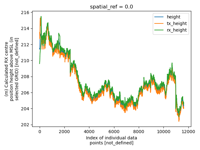
Plotting

plt.figure()
new_survey['data/raw_data']['height'].plot(label='height')
new_survey['data/raw_data']['tx_height'].plot(label='tx_height')
new_survey['data/raw_data']['rx_height'].plot(label='rx_height')
plt.tight_layout()
plt.legend()

plt.show()

Total running time of the script: (0 minutes 2.470 seconds)

Gallery generated by Sphinx-Gallery